You can create a FOCUS
report as one of several kinds of Microsoft Excel workbook.
EXL2K format generates styled reports in Excel
2000/2003 HTML format for use on other platforms and on the Web.
Feature options enable FOCUS users to also download all fields mentioned
in their requests in an Excel PivotTable, or include interactive
Excel formulas for FOCUS aggregation operations for performing additional
"what if" analyses on their data within Excel 2000/2003.
EXL97 is an HTML-based HOLD format for generating
formatted Excel 97 spreadsheets. EXL97 is a full StyleSheet driver
for accurately rendering all report elements (such as headings and
subtotals, for example) as well as applying StyleSheet syntax (such as,
conditional styling). You must have Microsoft Excel 97 or higher
installed on your computer to display an Excel 97 report.
xAssigning EXL2K Format to Your Report Output
The command ON TABLE HOLD
FORMAT EXL2K generates a fully styled Excel report in your browser,
with conditional styling capability.
The EXL2K (Excel 2000/2003) format is a full StyleSheet driver
that renders all report elements (for example, headings and subtotals)
as well as StyleSheet syntax (such as, conditional styling).
EXL2K format accurately displays formatted dates and numeric
values and controls column width and wrapping in Excel 2000/2003.
See Displaying Formatted Numeric Values in EXL2K Report Output, Passing FOCUS Dates to Excel 2000/2003 and Controlling Column Width and Wrapping in EXL2K Report Output.
In addition, the format variation EXL2K FORMULA enables you to
convert summed information (such as column totals, row totals, subtotals)
and calculated values to interactive formulas in an Excel 2000/2003
worksheet. See Generating Native Excel Formulas in EXL2K Report Output. Another format
variation, EXL2K PIVOT, enables you to analyze different views of
your data. See Using PivotTables in EXL2K Report Output.
EXL2K is supported only in Excel 2000 or 2003. It does not work
with any previous releases of Excel. You can invoke format EXL2K
reports using any browser supported by FOCUS.
By default, when you choose EXL2K as your display format, the
report opens in an Excel 2000/2003 worksheet, identified in a tab
at the bottom of the worksheet as Sheet1, Sheet2,
and so on. You can change the name of a Sheet tab to make it more
descriptive of your report's content.
Example: Creating an EXL2K Report
The
following example illustrates how to create a report in EXL2K (Excel
2000/2003) format with a styled heading, conditional styling on
SALES, and drill-downs on COUNTRY:
TABLE FILE CAR
HEADING
"SALES BY COUNTRY"
SUM SALES BY COUNTRY BY CAR BY MODEL
WHERE (COUNTRY EQ 'ENGLAND') OR (COUNTRY EQ 'ITALY') OR (COUNTRY EQ
'FRANCE');
ON TABLE HOLD FORMAT EXL2K
ON TABLE SET STYLE *
TYPE=REPORT, FONT=ARIAL, TITLETEXT=SALES REPORT, $
TYPE=DATA, COLUMN=COUNTRY, FOCEXEC=DRILLFEX (PARAM1=COUNTRY PARAM2=CAR),$
TYPE=DATA, COLUMN=SALES, COLOR=RED, BACKCOLOR=YELLOW, WHEN=SALES GT
10000,$
TYPE=DATA, COLUMN=MODEL, BACKCOLOR=YELLOW, WHEN=SALES GT 10000,$
TYPE=HEADING, FONT=ARIAL BLACK, COLOR=RED, BACKCOLOR=SILVER, SIZE=16, $
TYPE=TITLE, FONT=ARIAL, SIZE=12, $
ENDSTYLE
END
The output is:
Notice that the tab
name has been changed from the Excel default, Sheet1, to a more descriptive
name, which is specified in the TITLETEXT attribute of the StyleSheet.
For details on the TITLETEXT attribute see Customizing Tabular Reports.
x
Syntax: How to Create a Styled EXL2K File
[ON TABLE] HOLD [AS filename] FORMAT EXL2K [PIVOT] [FORMULA]
where:
- EXL2K
-
Creates an Excel-formatted output file that may include styling
based on internal or external StyleSheets features. The extension
on Windows platforms is .xht;
- PIVOT
-
Creates an output file in Excel PivotTable format with an
accompanying PivotTable cache file. The filetype of the Pivot Table
file is XML; the extension on Windows platforms is .xml. For more
information about this option, see Using PivotTables in EXL2K Report Output.
- FORMULA
-
Creates an XHT output file including appropriate Excel formulas
for all FOCUS numeric summary operations. For more information about
this option, see Generating Native Excel Formulas in EXL2K Report Output.
x
National Language Support With EXL2K
Excel 2000/2003 users can select one of six languages
as their default language when generating EXL2K formatted output.
In addition to English, which is the automatic default, users can
issue a SET command to select one of five other options.
x
Syntax: How to Set the Default Language
SET EXL2KLANG=lang
where:
-
lang
-
Is one of the following: AME, FRE, SPA, GER, JPN or KOR.
You
can code the SET EXL2KLANG in your user profile or include it in
a FOCEXEC to override the default setting in the NLSCFG ERRORS file
for a specific request.
x
Identifying Null Values in EXL2K Output Files
When an EXL2K report is run, and null values are retrieved
for one or more fields, blank spaces are displayed by default in
each cell of the report output for the empty (null) fields. This
behavior is the result of SET EMPTYCELLS ON being set by default
in the background of all EXL2K reports. If you want to identify
null values with something other than blank spaces, a character
string can be used to populate all empty fields in a report.
x
Syntax: How to Identify Null Values in EXL2K Reports
To
identify null values in EXL2K reports, use
ON TABLE SET NODATA character_string
ON TABLE SET EMPTYCELLS [ON|OFF]
where:
- character_string
- Is the string of characters displayed in the cells of the report
for each field where null values are retrieved from the database.
The maximum number of characters is 11. If the number of characters
in the string exceeds the length of the output field, the additional
characters will not be displayed. If special characters are used,
the string must be enclosed in single quotes. SET EMPTYCELLS OFF
must also be specified to make the SET NODATA command effective.
- ON
- Indicates that empty spaces are displayed in the cells of the
report for each field where null values are retrieved from the database.
ON is the default.
- OFF
- Indicates that zeros, or the character string specified with
the SET NODATA command, will be displayed in the cells of the report
for each field where null values are retrieved from the database.
OFF must be specified when using SET NODATA.
Example: Identifying Null Values in EXL2K Report Output
The
following syntax utilizes the default behavior of ON TABLE SET EMPTYCELLS
ON, which is set in the background:
TABLE FILE CAR
SUM SALES BY COUNTRY ACROSS SEATS
ON TABLE HOLD FORMAT EXL2K
END
The following output displays empty spaces in
the cells of the report for each field where null values are retrieved
from the database:
The following syntax
utilizes the SET NODATA command:
TABLE FILE CAR
SUM SALES BY COUNTRY ACROSS SEATS
ON TABLE SET NODATA 'n/a'
ON TABLE SET EMPTYCELLS OFF
ON TABLE HOLD FORMAT EXL2K
END
Note: If you do not add SET EMPTYCELLS
OFF, the SET NODATA command will be ignored.
The following
output displays 'n/a' in the cells of the report for each field
where null values are retrieved from the database:
The following syntax
turns off the default SET EMPTYCELLS behavior and does not use SET
NODATA, which makes it impossible to distinguish null values from
zero quantities:
TABLE FILE CAR
SUM SALES BY COUNTRY ACROSS SEATS
ON TABLE SET EMPTYCELLS OFF
ON TABLE HOLD FORMAT EXL2K
END
The following output displays zeros in the cells
of the report for each field where either null values are retrieved
from the database or the quantity is zero:
x
Displaying Formatted Numeric Values in EXL2K Report Output
Excel 2000/2003 workbooks generated by FOCUS EXL2K format contain the
numeric formatting specified in the Master File for the data source
or in a temporary field. FOCUS
numeric values (such as currency) are translated to supported Excel
formats and display properly in Excel 2000/2003.
When translating numeric formats from FOCUS
to Excel, there must be a corresponding Excel format to translate
to. If there is no corresponding format, then the value will be
formatted in the closest matching Excel format or in Excel General
format. For details, see Usage Notes for Numeric Formats.
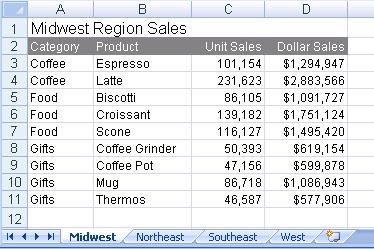
Example: Displaying Formatted Numeric Data in EXL2K Report Output
The
following example illustrates how formatted numeric data displays
in a worksheet when using the EXL2K format. Note that the format
for the Sales field
(D16.2M—which represents floating point double-precision with two
decimal places and a floating dollar sign) is translated to the corresponding
Excel format.
DEFINE FILE GGSALES
NEWDOLL/D16.2M = DOLLARS;
END
SET PAGE-NUM=OFF
TABLE FILE GGSALES
"Dollar Sales"
"Excel 2000 Spreadsheet"
" "
SUM NEWDOLL AS 'Sales'
BY REGION AS 'Area'
BY CATEGORY
BY PRODUCT
WHERE REGION EQ 'Midwest' OR 'Northeast'
ON TABLE SET BYDISPLAY ON
ON TABLE HOLD AS EXL2KNUM FORMAT EXL2K
ON TABLE SET STYLE *
TYPE=REPORT, GRID=OFF, FONT=TAHOMA, $
TYPE=HEADING, SIZE=14, COLOR=NAVY, $
TYPE=HEADING, LINE=2, SIZE=12, COLOR=RED, $
TYPE=TITLE, JUSTIFY=CENTER, STYLE=BOLD, $
TYPE=DATA, JUSTIFY=CENTER, $
TYPE=DATA, COLUMN=NEWDOLL, JUSTIFY=RIGHT, $
END
The output
is:
Notice that the values of
the sort fields are repeated in the output; this presentation, which
is particularly desirable in a worksheet, is controlled by the command
ON TABLE SET BYDISPLAY ON. For details, see Sorting Tabular Reports.
x
Reference: Usage Notes for Numeric Formats
The following formats are not supported
in EXL2K. They will translate into Excel General format and possibly
produce unpredictable results:
- Fixed Dollar (N) formats.
- Multiple format options. Only single format options are supported
when using FORMAT EXL2K. For example, the formats I9C and I9B are
supported, but I9BC is not.
The following applies to
headings and footings with embedded numeric fields:
- If you embed a numeric field in a heading, subheading, footing,
or subfooting of a report in an EXL2K report, the numeric field
displays in Excel general format (text). To display a numeric field
in Excel number format, you must set HEADALIGN=BODY in the StyleSheet.
x
Passing FOCUS Dates to Excel 2000/2003
Excel 2000/2003 workbooks generated by FOCUS EXL2K format contain the
numeric formatting specified in the Master File for the data source
or in a temporary field. FOCUS
date formats (such as Smart Dates) are translated to supported Excel
formats and display properly in Excel 2000/2003.
When translating date formats from FOCUS
to Excel, there must be a corresponding Excel format to translate
to. If there is no corresponding format, then the value will be
formatted in the closest matching Excel format or in Excel General
format. For details, see Usage Notes for Date Formats.
By default, when FOCUS creates
dates in Excel 2000 (EXL2K) format, the date formats that contain
translated values such as month or day name are sent as formatted
text, preserving the style defined for the report field. Numeric
dates are passed to Excel 2000/2003 as standard date values, not
as text. For information about passing translated date formats to
Excel 2000/2003 as date values with format masks, see Passing Dates With Translated Text to Excel 2000/2003.
Example: Displaying Formatted Dates in EXL2K Report Output
The
following example illustrates how customized dates display in a
worksheet when using the EXL2K format.
- The format
for Month Hired is defined in the request as
MtYY (the month is represented as a 3-character abbreviation with
an initial capital letter followed by a four-digit year).
- The format for Years of Service is defined
as I4C, a four-digit integer with a comma if required. Both formats
are properly displayed as defined in the worksheet.
SET PAGE-NUM=OFF
DEFINE FILE EMPLOYEE
YRHIRED/YY = HIRE_DATE;
MHIRED/MtYY = HIRE_DATE;
TOTSVC/I4C = 2002 - YRHIRED;
END
TABLE FILE EMPLOYEE
"Employee Service Report for 2002"
"Excel 2000 Spreadsheet"
" "
PRINT FIRST_NAME AS 'First Name'
MHIRED AS 'Month Hired'
TOTSVC AS 'Years of Service'
BY LAST_NAME AS 'Last Name'
ON TABLE SET BYDISPLAY ON
ON TABLE HOLD FORMAT EXL2K
ON TABLE SET STYLE *
TYPE=REPORT, GRID=OFF, FONT=TAHOMA, $
TYPE=HEADING, SIZE=14, COLOR=NAVY, $
TYPE=HEADING, LINE=2, SIZE=12, COLOR=RED, $
TYPE=TITLE, JUSTIFY=CENTER, STYLE=BOLD, $
TYPE=DATA, JUSTIFY=CENTER, $
TYPE=DATA, COLUMN=TOTSVC, COLOR=BLUE, WHEN=TOTSVC GT 20, $
END
The output is:
The command ON TABLE
SET BYDISPLAY ON ensures that sort fields are repeated in each worksheet
cell. For details, see Sorting Tabular Reports.
x
Reference: Usage Notes for Date Formats
The following formats are not supported
in EXL2K. They will translate into Excel General format and possibly
produce unpredictable results:
- YY, Y, M, D, JUL, and I2MT.
- Any date format with a Q (quarter).
- Any packed-decimal (P) date formats.
- Any alphanumeric (A) date formats.
x
Reference: Using Date Separators in Excel
In
order to use a "-" as a separator between month, day, and year in
Excel 2000/2003, you must change the default date separator for
Windows. This setting can be located under Regional Options in the
Control Panel.
x
Passing Dates With Translated Text to Excel 2000/2003
Some translated dates can be sent to Excel 2000/2003
as standard date values with format masks, enabling Excel to use
them in functions, formulas, and sort sequences. The SET EXL2KTXTDATE
command allows you to specify that translated dates should be sent
as date values with format masks instead of text values.
x
Syntax: How to Pass Translated Dates to Excel 2000/2003 as Date Values
SET EXL2KTXTDATE = {TEXT|VALUE}where:
- TEXT
- Passes date values that contain text to Excel 2000/2003 as formatted
text. TEXT is the default value.
- VALUE
- Passes the types of translated date values that contain text
and are supported Excel date formats to Excel 2000/2003 as standard
date values with text format masks applied.
x
Reference: Usage Notes for SET EXL2KTXTDATE
- The following date formats are not supported in EXL2K. They
will translate into Excel General format and possibly produce unpredictable
results:
- JUL, YYJUL, and I2MT.
- Dates stored as a packed or alphanumeric field with date display options.
- Excel only supports mixed-case, not all uppercase or all lowercase
for text dates. When EXL2KTXTDATE is set to VALUE, all FOCUS date formats containing text
will present in EXL2K as mixed-case, regardless of the casing parameters
defined in the FOCUS format. For example, MTRDY will
generate the date string JANUARY 2, 10 in standard FOCUS, but when sent to EXL2K as
a date value, it will be presented as January 2, 10.
Example: Passing Dates With Translated Text to Excel 2000/2003
The following request against the GGSALES
data source creates the date January 1, 2010 and converts it to
four date formats with translated text:
SET EXL2KTXTDATE=TEXT
DEFINE FILE GGSALES
NEWDATE/MDYY = '01/01/2010';
WRMtrDY/WRMtrDY = NEWDATE;
wDMTY/wDMTY= NEWDATE;
wrDMTRY/wrDMTRY= NEWDATE;
wrYMtrD/wrYMtrD= NEWDATE;
END
TABLE FILE GGSALES
SUM DATE NOPRINT
NEWDATE WRMtrDY wDMTY wrDMTRY wrYMtrD
ON TABLE HOLD FORMAT EXL2K
END
The following table shows
how the dates should appear with EXL2KTXTDATE set to TEXT and to
VALUE.
FOCUS Format | SET EXL2KTXTDATE=TEXT | SET EXL2KTXTDATE=VALUE |
|---|
EXL2K Displays: | EXL2K Value: | EXL2K Displays: | EXL2K Value: |
|---|
WRMtrDY | FRIDAY, January 1 10 | FRIDAY, January 1 10 | Friday, January 1 10 | 1/1/2010 |
wDMTY | Fri, 1 JAN 10 | Fri, 1 JAN 10 | Fri, 1 Jan 10 | 1/1/2010 |
wrDMTRY | Friday, 1 JANUARY 10 | Friday, 1 JANUARY 10 | Friday, 1 January 1 | 1/1/2010 |
wrYMtrD | Friday, 10 January 1 | Friday, 10 JANUARY 1 | Friday, 10 January 1 | 1/1/2010 |
With SET EXL2KTXTDATE=TEXT,
in EXL2K report output all the cells with month or day translation
are sent as text, and all month and day names are in the case specified
by the FOCUS format. The output
is:

With
SET EXL2KTXTDATE=VALUE, in EXL2K report output all of the cells
have a date value with format masks, and all month and day names
are in mixed-case, regardless of how the case has been specified
in the FOCUS format. The output
is:

x
Passing Dates Without a Day Component
Date formats that do not specify the day value explicitly
are defined as the date value of the first day of the month. Therefore,
the value placed in the cell may be different from the day component
value in the source data field and may produce unexpected results
when used for sorting or date calculations in an Excel formula.
The following table shows how FOCUS date formats are represented in
EXL2K report output. The table shows how the value is preserved
in the cell and how the display is generated using the format mask
that corresponds to the FOCUS date
format.
DATEFLD/MDYY = '01/02/2010'
FOCUS Format | SET EXL2KTXTDATE=TEXT | SET EXL2KTXTDATE=VALUE |
|---|
EXL2K Displays: | EXL2K Value: | EXL2K Displays: | EXL2K Value: |
|---|
DMYY | 02/01/2010 | 1/2/2010 | 02/01/2010 | 1/2/2010 |
MY | 01/10 | 1/1/2010 | 01/10 | 1/1/2010 |
MTY | JAN, 10 | JAN, 10 | Jan, 10 | 1/1/2010 |
MTDY | JAN 2, 10 | JAN 2, 10 | Jan 2, 10 | 1/2/2010 |
Example: Passing FOCUS Dates With and Without a Day Component to Excel 2000/2003
The following request against the GGSALES
data source creates the date January 2, 2010 and passes it to Excel
2000/2003 with formats MDYY, DMYY, MY, and MTDY:
SET EXL2KTXTDATE=TEXT
DEFINE FILE GGSALES
NEWDATE/MDYY = '01/02/2010';
END
TABLE FILE GGSALES
SUM DATE NOPRINT
NEWDATE AS 'MDYY' NEWDATE/DMYY AS 'DMYY' NEWDATE/MY
AS 'MY' NEWDATE/MTY AS 'MTY' NEWDATE/MTDY AS 'MTDY'
ON TABLE HOLD FORMAT EXL2K
ENDWith EXL2KTXTDATE=TEXT,
columns D and E have a text values, not date values. The values
are displayed in uppercase as specified by the FOCUS
formats (MTY and MTDY):
With
EXL2KTXTDATE=VALUE, columns D and E have actual date values with
format masks, displayed by Excel 2000 in mixed-case. Since the MTY
format does not have a day component, the date value stored is the
first of January 2010 (1/1/2010), not the second of January 2010
(1/2/2010):
x
Passing Date Components for Use in EXL2K FORMULA Reports
Dates formatted as individual components (for example,
D, Y, M, W) are passed to Excel 2000/2003 as numeric values that
can be used as parameters to Excel date functions. The values are
passed as general text format that are recognized by Excel 2000/2003
as numbers. These values are passed to Excel in the same format
regardless of the setting for EXL2KTXTDATE.
Example: Passing Numeric Date Components to Excel 2000/2003
The following request against the GGSALES
data source creates the date January 1, 2010 and extracts numeric
date components, passing them to Excel 2000/2003:
SET EXL2KTXTDATE=VALUE
DEFINE FILE GGSALES
NEWDATE/MDYY = '01/01/2010';
D/D= NEWDATE;
Y/Y = NEWDATE;
W/W=NEWDATE;
w/w=NEWDATE;
M/M = NEWDATE;
YY/YY = NEWDATE;
END
TABLE FILE GGSALES
SUM DATE NOPRINT
NEWDATE D Y W w M YY
ON TABLE HOLD FORMAT EXL2K
END
With SET EXL2KTXTDATE=VALUE,
the output is:
x
Date formats that contain a Quarter component are always
passed to Excel as text strings since Excel does not support Quarter
formats.
Example: Passing Dates With a Quarter Component to Excel 2000/2003
The following request against the GGSALES
data source creates the date January 1, 2010 and converts it to
date formats that contain a Quarter component:
SET EXL2KTXTDATE=VALUE
DEFINE FILE GGSALES
NEWDATE/MDYY = '01/01/2010';
Q/Q= NEWDATE;
QY/QY = NEWDATE;
YBQ/YBQ=NEWDATE;
END
TABLE FILE GGSALES
SUM DATE NOPRINT
NEWDATE Q QY YBQ
ON TABLE HOLD FORMAT EXL2K
END
Even with SET EXL2KTXTDATE=VALUE, in the EXL2K
report output, the cells containing dates with Quarter components
have General format. To see this, open the Format Cells dialog box.
The output is:
x
Passing Date Components Defined as Translated Text
Date formats that do not contain
sufficient information to present the valid date result in Excel
are not translated to a value, including formats that do not contain
year and/or month information. These dates will continue to be sent
to Excel 2000/2003 as text regardless of the SET EXL2KTXTDATE setting.
In the absence of complete information, the year defaults to the
current year, so the value sent would be incorrect if this type
of format was passed as a date value. The following formats will
not be sent as values:
- MT, MTR, Mt, Mtr
- W, w, WR, wr
Note that since these values are always sent as text, the casing
defined in the FOCUS format is
applied in the resulting cell.
Example: Passing Date Components Defined as Translated Text to Excel 2000/2003
The following request against the GGSALES
data source creates the date January 1, 2010 and converts it to
date formats that are defined as either month name or day name:
SET EXL2KTXTDATE=VALUE
DEFINE FILE GGSALES
NEWDATE/MDYY = '01/01/2010';
MT/MT= NEWDATE;
MTR/MTR= NEWDATE;
Mtr/Mtr = NEWDATE;
WR/WR = NEWDATE;
wr/wr = NEWDATE;
END
TABLE FILE GGSALES
SUM DATE NOPRINT
NEWDATE MT MTR Mtr WR wr
ON TABLE HOLD FORMAT EXL2K
END
In Excel 2000/2003, the cells containing the days
have General format. To see this, open the Format Cells dialog box.
The output is:
x
Controlling Column Width and Wrapping in EXL2K Report Output
Data wrapping, column width, and the scroll area can
be controlled in an Excel 2000/2003 worksheet when using FORMAT
EXL2K. You can:
- Turn data wrapping on. The default behavior is for all data
to wrap according to a default column width that is determined by
Excel.
- Turn data wrapping off. This setting allows columns to expand
to the length of the data value. The column width is determined
by Excel, but should be wide enough to fit the longest data value
in the column. If a portion of the data is hidden, you can adjust the
column width in Excel after the worksheet has been generated.
- Turn data wrapping off and set the column width at the same
time. If a data value is wider than the specified width of the column,
a portion of the data will be hidden from view. You can adjust the
column width in Excel after the worksheet has been generated.
- Specify the exact width of a column with data wrapping on.
x
Syntax: How to Wrap Data in EXL2K Report Output
TYPE=REPORT, [COLUMN=column,] WRAP=value, $
where:
- column
- Designates a particular column to apply wrapping behavior to.
If COLUMN is not included in the declaration, wrapping will be applied
to the entire report.
- value
- Is one of the following:
- ON
- Turns on data wrapping. ON is the default value. With this setting,
the column width is determined by the client (Excel). Data wraps
if it exceeds the width of the column and the row's height expands
to meet the new height of the wrapped data.
- OFF
- Turns off data wrapping. This setting adjusts the column width
of the largest data value in the column. Data will not wrap in any
cell in the column.
- n
- Represents a specific numeric value that the column width can
be set to. The value represents the measure specified with the UNITS
parameter (the default is inches).
This setting implies ON. However,
the column width is set to the specified width unless the data is
wider than the column width, in which case, wrapping will occur
as for ON.
x
Syntax: How to Set Column Width in EXL2K Report Output
TYPE=REPORT, [COLUMN=column,] SQUEEZE={ON|OFF|n}, $where:
- column
- Identifies a particular column. If COLUMN is not included in
the declaration, default SQUEEZE behavior is applied to the entire
report.
- n
- Represents a specific numeric value that the column width can
be set to. The value represents the measure specified with the UNITS
parameter (the default is inches).
This is the most commonly used
SQUEEZE setting in an EXL2K report.
Note:
- ON/OFF settings for SQUEEZE are not meaningful for EXL2K, and
both produce the default behavior.
- SQUEEZE = n turns off data wrapping. If a data value
is wider than the specified width of the column, it is hidden from
view. You can adjust column width in Excel after the worksheet has
been generated.
- SQUEEZE is not supported for columns created with the OVER phrase.
Example: Controlling Column Width and Wrapping in EXL2K Report Output
The
following example illustrates how to turn on and turn off data wrapping
in a column and how to set the column width for a particular column.
The UNITS in this example are set to inches (the default).
DEFINE FILE CAR
MYDATE/MDY='10/22/60';
RCD/D14.3=RETAIL_COST;
VERYLONG/A80='Subtract dealer cost from retail cost to calculate
profit.';
END
TABLE FILE CAR
PRINT MYDATE RCD
VERYLONG AS 'Default' VERYLONG AS 'WRAP=OFF'
VERYLONG AS 'WRAP=4.1' VERYLONG AS 'WRAP=2'
VERYLONG AS 'SQUEEZE=2' SALES
BY COUNTRY
ON TABLE HOLD FORMAT EXL2K
ON TABLE SET STYLE *
TYPE=DATA, COLUMN=MYDATE, JUSTIFY=CENTER, $
1. TYPE=REPORT, COLUMN=VERYLONG(2), WRAP=OFF, $
2. TYPE=REPORT, COLUMN=VERYLONG(3), WRAP=4.1, $
3. TYPE=REPORT, COLUMN=VERYLONG(4), WRAP=2, $
4. TYPE=REPORT, COLUMN=VERYLONG(5), SQUEEZE=2, $
END
where:
- Identifies the column titled "WRAP=OFF" and turns off data wrapping
for that column.
- Identifies the column titled "WRAP=4.1" and sets the column
width to 4.1 inches with data wrapping on.
- Identifies the column titled "WRAP=2" and sets the column width
to 2 inches with data wrapping on.
- Identifies the column titled "SQUEEZE=2" and sets the column
width to 2 inches with data wrapping off.
Note: The
column titled "Default" illustrates the default column width and wrapping
behavior.
Since the output is wider than this page, it is
shown in two sections. The following output displays the "Default",
"WRAP=OFF", and "WRAP=4.1" columns:
The following output
displays the "WRAP=2", and "SQUEEZE=2" columns:
x
Locking Columns in EXL2K Report Output
Using StyleSheet attributes, you can lock Excel workbook
values so they are read-only. These attributes apply to all EXL2K
formats including EXL2K, EXL2K PIVOT, and EXL2K FORMULA.
x
Syntax: How to Enable Worksheet Locking
To enable locking, use the following attributes:
TYPE=REPORT, PROTECTED={ON|OFF}, [LOCKED={ON|OFF}],$where:
- TYPE=REPORT,
PROTECTED=ON
- Is necessary to enable worksheet locking. PROTECTED=OFF is
the default. If you omit the LOCKED=OFF attribute, the entire worksheet
is locked.
- LOCKED=ON
- Locks the entire worksheet. ON is the default value.
- LOCKED=OFF
- Unlocks the worksheet as a whole, but enables you to lock or
unlock specific cells or groups of cells.
x
Syntax: How to Lock Specific Cells Within a Worksheet
Once you include the following declaration
in your StyleSheet, you can specify the LOCKED attribute for specific
cells or groups of cells:
TYPE=REPORT, PROTECTED=ON, LOCKED=OFF,$
To lock specific parts of the worksheet,
add the LOCKED=ON attribute to the StyleSheet declaration for the
cells you want to lock.
TYPE=type, [ COLUMN=columnspec ] ,LOCKED={ON|OFF},$where:
- type
- Is the type of element that describes the cells to be locked.
- columnspec
- Is a valid column specification.
Example: Locking an Entire EXL2K Workbook
The following request locks the entire
workbook because the StyleSheet declarations include the following
declaration:
TYPE=REPORT, PROTECTED=ON, $
The request is:
TABLE FILE CAR
HEADING
"Profit By Car "
" "
SUM RETAIL_COST AND DEALER_COST AND
COMPUTE PROFIT/D12.2 = RETAIL_COST - DEALER_COST;
BY CAR
ON TABLE SET PAGE-NUM OFF
ON TABLE HOLD AS EXLFORM1 FORMAT EXL2K
ON TABLE SET STYLE *
TYPE=REPORT, COLOR=BLUE, BACKCOLOR=SILVER, SIZE=9,$
TYPE=REPORT, PROTECTED=ON, $
TYPE=HEADING, STYLE=BOLD, SIZE=14, $
TYPE=TITLE, STYLE=BOLD, SIZE=11,$
ENDSTYLE
END
You cannot edit any value on the worksheet.
Any attempt to do so displays a message that the sheet is protected:
Example: Locking a Single Column on an EXL2K Workbook
The following request locks the second
column (RETAIL_COST) because the StyleSheet declarations include
the following declarations:
TYPE=REPORT, PROTECTED=ON, LOCKED=OFF, $
TYPE=DATA, COLUMN=2, LOCKED=ON,$
The
request is:
TABLE FILE CAR
HEADING
"Profit By Car "
" "
SUM RETAIL_COST AND DEALER_COST AND
COMPUTE PROFIT/D12.2 = RETAIL_COST - DEALER_COST;
BY CAR
ON TABLE SET PAGE-NUM OFF
ON TABLE HOLD AS EXLFORM2 FORMAT EXL2K
ON TABLE SET STYLE *
TYPE=REPORT, COLOR=BLUE, BACKCOLOR=SILVER, SIZE=9,$
TYPE=REPORT, PROTECTED=ON, LOCKED=OFF,$
TYPE=HEADING, STYLE=BOLD, SIZE=14, $
TYPE=TITLE, STYLE=BOLD, SIZE=11,$
TYPE=DATA, COLUMN=2, LOCKED=ON,$
ENDSTYLE
END
You cannot edit any value in column
2, although you can edit values in other columns. Any attempt to
edit a value in column 2 displays a message that the cells are protected:
x
Generating Native Excel Formulas in EXL2K Report Output
When you display or save a tabular report request using
EXL2K FORMULA, the resulting worksheet contains an Excel formula
that computes and displays the results of any type of summed information
(such as column totals, row totals, subtotals, and calculated values),
rather than static numbers. Worksheets saved using the EXL2K FORMULA
format are interactive, allowing for "what if" scenarios that immediately
reflect any additions or modifications made to the data.
The EXL2K FORMULA format is supported for the FOCUS TABLE commands: ROW-TOTAL,
COLUMN-TOTAL, SUB-TOTAL, SUBTOTAL, SUMMARIZE, RECOMPUTE, and COMPUTE,
and for calculations performed by functions. See Translation Support for FORMAT EXL2K FORMULA.
EXL2K FORMULA is not supported with PivotTables (EXL2K
PIVOT), with Excel 97 (EXL97), or with financial reports created
with the Financial Report Painter or the underlying Financial Modeling
Language (FML).
x
Syntax: How to Save Reports as FORMAT EXL2K FORMULA
Add
the following syntax to your request to take advantage of Excel
formulas in your workbook:
ON TABLE HOLD FORMAT EXL2K FORMULA
where:
- HOLD
- Saves the output for reuse in an Excel 2000/2003 worksheet.
For details, see Saving and Reusing Your Report Output.
Example: Generating Native Excel Formulas for Column Totals
The
following example illustrates the translation of a column total
in a report request into an Excel formula when using format EXL2K
FORMULA. Note that the formatting of the column total (TYPE=GRANDTOTAL)
is retained in the Excel 2000 spreadsheet.
When
you select the total in the report, the equation =SUM(B4:B7) appears
in the formula bar, representing the column total as a sum of cell
ranges.
TABLE FILE CENTORD
HEADING
"Projected Return By Region"
" "
SUM LINE_COGS AS 'RETURN'
BY REGION AS 'REGION'
ON TABLE COLUMN-TOTAL
ON TABLE HOLD AS EXL2K5 FORMAT EXL2K FORMULA
ON TABLE SET STYLE *
TYPE=REPORT, COLOR=BLUE, BACKCOLOR=SILVER, SIZE=9,$
TYPE=HEADING, STYLE=BOLD, SIZE=14,$
TYPE=TITLE, STYLE=BOLD+UNDERLINE, SIZE=10,$
TYPE=GRANDTOTAL, STYLE=BOLD,$
ENDSTYLE
END
The output is:
Example: Generating Native Excel Formulas for Row Totals
This
request calculates totals for line price and quantity across regions.
The row totals are represented as sums of cell ranges.
TABLE FILE CENTORD
HEADING
"Projected Line Cost Across Region"
" "
SUM LINEPRICE AND QUANTITY
ACROSS REGION AS 'Region'
BY STORENAME
WHERE REGION EQ 'EAST' OR 'NORTH'
ON REGION ROW-TOTAL AS 'TOTAL'
ON TABLE COLUMN-TOTAL AS 'TOTAL'
ON TABLE HOLD AS EXL2K6 FORMAT EXL2K FORMULA
ON TABLE SET STYLE *
TYPE=REPORT, COLOR=BLUE, BACKCOLOR=SILVER, SIZE=9,$
TYPE=HEADING, STYLE=BOLD, SIZE=14,$
TYPE=TITLE, STYLE=BOLD, SIZE=11,$
TYPE=SUBTOTAL, STYLE=BOLD, $
TYPE=GRANDTOTAL, STYLE=BOLD, SIZE=11,$
TYPE=ACROSSTITLE, STYLE=BOLD, SIZE=11, JUSTIFY=LEFT,$
TYPE=ACROSSVALUE, STYLE=BOLD, SIZE=10, JUSTIFY=CENTER,$
ENDSTYLE
END
The output highlights the formula that calculates
the row total in cell G11=C11+E11:
Example: Generating Native Excel Formulas for Calculated Values
This request totals the columns for
retail cost and dealer cost and calculates the value of a field
called PROFIT by subtracting the dealer cost from the retail cost.
The
formula for the calculated values is generated by translating the
internal form of the FOCUS expression
(COMPUTE PROFIT/D12.2 = RC - DC;) into an Excel formula. In this
example, the formulas appear in cells B14, C14, and D14.
TABLE FILE CAR
ON TABLE SET PAGE-NUM OFF
SUM RC AND DC AND
COMPUTE PROFIT/D12.2 = RC - DC;
BY CAR
HEADING
"Profit By Car"
" "
ON TABLE COLUMN-TOTAL
ON TABLE HOLD FORMAT EXLL2K FORMULA
ON TABLE SET STYLE *
TYPE=REPORT, COLOR=BLUE, BACKCOLOR=SILVER, SIZE=9,$
TYPE=HEADING, STYLE=BOLD, SIZE=14, $
TYPE=TITLE, STYLE=BOLD, SIZE=11,$
TYPE=GRANDTOTAL, STYLE=BOLD, SIZE=11,$
ENDSTYLE
END
The following output highlights
the formula that calculates for the column total of PROFIT: D14=SUM(D4:D13).
Example: Generating a Native Excel Formula for a Function
The
following illustrates how functions are translated to Excel 2000/2003
reports. The function DMOD divides ACCTNUMBER by 1000 and returns
the remainder to LAST3_ACCT. The Excel formula corresponds to this,
=TRUNC((MOD($C3,(1000)))).
TABLE FILE EMPLOYEE
PRINT ACCTNUMBER AS 'Account Number' AND COMPUTE
LAST3_ACCT/I3L = DMOD(ACCTNUMBER, 1000, LAST3_ACCT);
BY LAST_NAME AS 'Last Name'
BY FIRST_NAME AS 'First Name'
WHERE (ACCTNUMBER NE 000000000) AND (DEPARTMENT EQ 'MIS');
ON TABLE HOLD FORMAT EXL2K FORMULA
ON TABLE SET STYLE *
TYPE=TITLE, SIZE=12, STYLE=BOLD, $
END
The output is:
x
Reference: Generating a Formula With Recomputed Values
If
your report contains a calculated value (generated by the COMPUTE
or RECOMPUTE command), all of the fields referenced by the calculated
value must be displayed in the report in order for cell references
to be included in the formula. If a referenced column is not displayed
in the workbook, the data value will be placed in the formula, rather
than a cell reference. In the case of recompute, the value used
may be an incorrect value from the last detail record of the sort
break.
Example: Generating a Formula With Recomputed Values
The
following request computes the difference (DIFF) by subtracting
budgeted dollars from dollar sales. The budgeted dollars field used
in the expression is not included in the SUM command. The value
of DIFF is recomputed on the region level:
TABLE FILE GGSALES
HEADING
"Profit By Region"
" "
SUM DOLLARS
COMPUTE DIFF/I9=DOLLARS - BUDDOLLARS;
BY REGION
BY CATEGORY
ON REGION RECOMPUTE
ON TABLE HOLD FORMAT EXL2K FORMULA
END
The output shows that
the formula is subtracting a data value that is not displayed on the
worksheet. It is actually the BUDDOLLARS value from the previous
row:
If
you change the SUM command to the following, the formula can be
recomputed correctly:
SUM DOLLARS BUDDOLLARS
The formula generated with the new SUM
command contains cell references for both fields used in the calculation:
x
Reference: Translation Support for FORMAT EXL2K FORMULA
- All standard operators are supported.
These include arithmetic operators, relational operators, string
operators, IF/THEN/ELSE, and logical operators. However, column
notation is not supported.
The IS-PRESENT,
IS-MISSING, CONTAINS, and OMITS operators are not supported. In
addition the logical operators (AND, OR) are not supported within
IF/THEN/ELSE statements.
- The following functions are supported:
ABS,
ARGLEN, ATODBL, BYTVAL, CHARGET, CTRAN, CTRFLD, DECODE DMOD, DOWK,
DOWKI, DOWKL, DOWKLI, EDIT (1 argument variant only), EXP, EXPN,
FMOD, HEXBYT, HHMMSS, IMOD, INT, LCWORD, LJUST, LOCASE, LOG, MAX,
MIN, OVRLAY, POSIT, RDUNIF, RANDOM, RJUST, SQRT, SUBSTR, TODAY,
TODAYI, UPCASE, YM. The EDIT function is not supported for editing
strings.
If you use the COMPUTE command with an unsupported
function, an error message is displayed.
- EXL2K FORMULA is not supported with
the following FOCUS commands and phrases:
- DEFINE.
- OVER.
- FOR.
- NOPRINT.
- Multiple display (PRINT, LIST, SUM, and COUNT) commands.
- SEQUENCE StyleSheet attribute.
- RECAP.
- SET HIDENULLACRS.
- SET SUBTOTALS = ABOVE.
- LAST.
- If your report contains a calculated value (generated by the
COMPUTE or RECOMPUTE command), all of the fields referenced by the
calculated value must be displayed in the report in order for a
cell reference to be included in the formula. If the referenced
column is not displayed in the workbook, the data value will be
placed in the formula rather than a cell reference.
- Formulas for ROW-TOTALs are represented by addition of specific
cells, while formulas for COLUMN-TOTALs are represented as sums
of cell ranges. For example, =SUM(G2:G10).
- A formula for a calculated value is generated by translating
the internal form of the FOCUS
expression into an Excel formula.
- The setting BYDISPLAY ON is recommended, otherwise the sort
field value will not be available on all rows for recalculations.
- Excel 2000/2003 formulas are limited to 1024 characters. Therefore,
the translation to an Excel formula will fail if a FOCUS total or the result of an
expression requires more than 1024 bytes of Excel formula code,
and an error message will be generated.
- Conditional styling is based on the values in the original report.
If the worksheet values are changed and the formulas are recomputed,
the styling will not reflect the updated information.
x
Using EXL2K Formula With Prefix Operators
EXL2K FORMULA output supports
prefix operators that are used on summary lines generated by FOCUS commands,
such as SUBTOTAL and RECOMPUTE. Where a corresponding formula exists
in Excel, these prefix operators are translated into the equivalent
Excel summarization formula. The results of prefix operators used
directly against retrieved data continue to be passed to Excel as values,
not formulas.
The following table identifies the prefix
operators supported by EXL2K FORMULA when used on summary lines,
and the Excel formula equivalent placed in the generated worksheet.
|
Prefix Operator
|
Excel Formula Equivalent
|
|---|
|
SUM.
|
=SUM()
|
|
AVE.
|
=AVERAGE()
|
|
CNT.
|
=COUNT()
|
|
MIN.
|
=MIN()
|
|
MAX.
|
=MAX()
|
The following prefix operators are not
translated to formulas when used on summary lines in EXL2K FORMULA.
Note:
- When using a prefix operator
on a field specified directly against retrieved data, there is no
space between the prefix operator and the field on which it operates.
For example, in the following aggregating
display command, the AVE. prefix operator operates on the DEALER_COST
field:
SUM AVE.DEALER_COST
- When using a prefix operator on a summary line, you must leave
a space between the prefix operator and the aggregated field on
which it operates.
In the following summary
command, the MAX. prefix operator operates on the DOLLARS field
at the REGION sort break. Note the required blank space between
the prefix operator and the field name:
ON REGION RECOMPUTE MAX. DOLLARS
Example: Using a Summary Prefix Operator With Format EXL2K FORMULA
In the following request against the
GGSALES data source, the RECOMPUTE command for the REGION sort field
calculates the maximum of the aggregated DOLLARS field and the minimum
of the aggregated BUDDOLLARS field:
TABLE FILE GGSALES
SUM UNITS DOLLARS BUDDOLLARS
AND COMPUTE DIFF/I10= DOLLARS-BUDDOLLARS;
BY REGION
BY CATEGORY
WHERE CATEGORY EQ 'Food' OR 'Coffee'
WHERE REGION EQ 'West' OR 'Midwest'
ON REGION RECOMPUTE MAX. DOLLARS MIN. BUDDOLLARS DIFF
ON TABLE HOLD FORMAT EXL2K FORMULA
END
On the output, the
cell that represents the recomputed DOLLARS for the Midwest region
has been generated as the formula =MIN(E2:E3).
x
Using PivotTables in EXL2K Report Output
The power of EXL2K format derives in large measure from
its ability to take advantage of PivotTables. The PivotTable is
a tool used in Microsoft Excel to analyze complex data.
It allows you to drag data fields within a PivotTable, providing
different views of the data, such as sorting across rows or columns.
You can also create dimensional hierarchies, similar to those created
using WITHIN syntax, by using the PAGEFIELDS command.
Report requests can be created in FOCUS
and sent as output to a fully formatted Excel PivotTable. The ON
TABLE HOLD FORMAT EXL2K PIVOT command
will generate an Excel PivotTable in your browser.
When FORMAT EXL2K PIVOT is enabled, two
data streams are created:
- The first data stream is the PivotTable
file.
The PivotTable file (.xht) is an HTML file with embedded
XML. The HTML file contains all the information that is displayed
in your browser.
- The second data stream is the PivotTable cache file (.xml).
The
PivotTable cache file is a metadata type of file. It contains all
the fields specified in the procedure and links internally to the
PivotTable file. The PivotTable cache file can contain data fields
called CACHEFIELDS, which populate the PivotTable toolbar, but do
not initially display in the report. CACHEFIELDS can be dragged
and dropped from the PivotTable toolbar into the PivotTable when
required for analysis. The two data streams are packaged into one
output file when the WEBARCHIVE parameter is set to ON. ON is the
WEBARCHIVE parameter default value.
After creating FOCUS reports formatted as Excel
PivotTables you must transfer both the XHT and XML files to Excel
2000 using FTP in ASCII mode or another transfer facility.
x
Procedure: How to View the PivotTable Toolbar in Excel 2000/2003
The
PivotTable toolbar may not automatically display when a PivotTable
is created. To display the PivotTable toolbar, use the following
procedure:
-
Click View in the Excel toolbar.
-
Highlight Toolbars.
-
Click PivotTable.
Excel 2000/2003 displays the PivotTable toolbar, listing
the fields available to be dragged into the body of the PivotTable
report. A cell within the PivotTable must be selected for the Pivot
toolbar to display all fields.
x
Reference: How TABLE Elements Appear in a Pivot Table
The
PivotTable is generated by the PRINT command in combination with
the BY, ACROSS, PAGEFIELDS and CACHEFIELDS phrases. It contains
all options used to design and format the report, as well as fields
specified in the PIVOT request. Fields can be dragged into the report
from the toolbar. The following graphic depicts PivotTable output
with the major elements identified.
The following summary
table shows PivotTable elements and the associated FOCUS syntax.
|
PivotTable Element
|
Contains...
|
Function
|
Generating Syntax
|
|---|
|
Page field
|
Field that controls view of the entire page (worksheet).
|
A filtering mechanism to conduct a high
level sort.
|
PAGEFIELDS phrase
|
|
Page field item
|
The value for a page field item displays in
a drop-down list.
|
Selecting a page field item summarizes data
for the entire report.
|
PAGEFIELDS phrase
|
|
Data field
|
Numeric data that is available to be summarized.
|
Holds data available to be summarized.
|
PRINT command
|
|
Column field
|
Horizontal sort data.
|
Sorts data horizontally.
|
ACROSS command
|
|
Row field
|
Vertical sort data.
|
Sorts data vertically.
|
BY command
|
x
Reference: Effect of TABLE Syntax Elements on PivotTables
The
following table summarizes TABLE syntax elements that are supported
in EXL2K PIVOT. The effect of each command on your PivotTable request
is listed, along with required usage.
|
Syntax Element
|
Usage
|
Effect on PivotTable
|
|---|
|
PRINT
|
Required.
|
Designates the data field in a PivotTable.
|
|
BY
|
Optional. *
|
Designates row field in a PivotTable.
|
|
ACROSS
|
Optional. *
|
Designates a column field in a PivotTable.
|
|
CACHEFIELDS
|
Optional. *
|
Places fields in the Pivot cache file and makes
them available from the Pivot toolbar.
|
|
PAGEFIELDS
|
Optional. *
|
Designates a Page field in a PivotTable.
|
* You need at least one sort field or a PAGEFIELD
for a valid Pivot Table.
x
The standard HOLD and SAVE syntax for storing the output
file on disk is supported for the EXL2K PIVOT file format. When
FORMAT EXL2K PIVOT is enabled, two files are created, the PivotTable
file (.xht) and a PivotTable cache file (.xml). The PivotTable cache file
contains all the fields specified in the procedure and links internally
to the PivotTable file. All available fields can be viewed in the
PivotTable toolbar.
You can include the CACHEFIELDS phrase in a request to add fields
to the pivot cache that are not initially displayed in the report.
The cache file enables you to add available fields from the PivotTable
toolbar into the body of the PivotTable by dragging and dropping.
You can remove fields from the PivotTable by dragging and dropping
them anywhere outside the report. Using these tools, you can quickly
vary data views.
x
Syntax: How to Enable the PivotTable
The
following are syntax variations that you can use to enable FORMAT
EXL2K PIVOT.
ON TABLE HOLD FORMAT EXL2K PIVOT AS mypivot
where:
- mypivot
- Is a name you assign to the HOLD file.
Two files are generated with this syntax:
- MYPIVOT.XHT is the main file that is displayed
in the browser or Excel window.
- MYPIVO$.XML is the Pivot Cache file.
x
Reference: Usage Notes for PivotTable Requests
You should consider the following when
writing requests for output to a PivotTable:
Example: Using the EXL2K PIVOT Option
This
simple example shows how to populate and generate PivotTables:
TABLE FILE CENTINV
HEADING
"CENTINV File PivotTable"
"Sum of Price by Product Across Category"
PRINT PRICE
BY PROD_NUM
ACROSS PRODCAT
ON TABLE COLUMN-TOTAL
ON TABLE HOLD AS EXL2K9 FORMAT EXL2K PIVOT
PAGEFIELDS PRODNAME
CACHEFIELDS COST QTY_IN_STOCK
ON TABLE SET STYLE *
TYPE=HEADING, LINE=1, FONT='ARIAL', COLOR=PURPLE, SIZE=16, STYLE=BOLD,$
TYPE=HEADING, LINE=2, FONT='ARIAL', COLOR=PURPLE, SIZE=12, STYLE=BOLD,$
TYPE=DATA, FONT='ARIAL', COLOR=PURPLE,$
TYPE=GRANDTOTAL, FONT='ARIAL', COLOR=PURPLE, SIZE=12, STYLE=BOLD,$
ENDSTYLE
END
The output is:
x
Designating CACHEFIELDS in PivotTables
You can specify multiple fields as CACHEFIELDS. These
fields will not initially display in the report, but will be available
in the pivot cache file if you wish to include them in the report
at a later time.
You can then drag these fields in and out of the PivotTable as
desired. CACHEFIELDS is an optional phrase; you can generate a PivotTable
without a CACHEFIELD.
x
Reference: Usage Notes for Specifying CACHEFIELDS
Fields
designated as CACHEFIELDS must be placed immediately after the PIVOT
keyword in the ON TABLE HOLD FORMAT
EXL2K PIVOT syntax or after a PAGEFIELDS phrase. A field specified
as a CACHEFIELD cannot be designated anywhere else in the request.
A list of CACHEFIELDS is terminated by the same keywords that terminate
a normal report request, such as END or another ON phrase.
Example: Using CACHEFIELDS With EXL2K PIVOT
This
example shows how to specify CACHEFIELDS to populate the PivotTable toolbar.
TABLE FILE CENTINV
HEADING
"PivotTable with CACHEFIELDS"
"Sum of Price by Product Across Category"
PRINT PRICE
BY PRODCAT BY PRODTYPE
ON PRODCAT SUB-TOTAL
ON TABLE HOLD AS EXL2K10 FORMAT EXL2K PIVOT
CACHEFIELDS COST PRODNAME
ON TABLE SET STYLE *
TYPE=DATA, COLUMN=PRODCAT, COLOR=RED,$
TYPE=HEADING, COLOR=BLUE, STYLE=BOLD, SIZE=14,$
ENDSTYLE
END
The output is:
x
Designating PAGEFIELDS in PivotTables
You can specify a field in the procedure as an Excel
2000/2003 page field. The page field filters the data for the specified
field. Then, using PivotTable functionality, you can choose a single
value from the page field drop-down menu (also called a page field
item) and immediately see only the data associated with that selection.
For example, in a report that shows international sales data for
cars, if you specify COUNTRY as your page field and select JAPAN
as your page field item, you will see only sales data for TOYOTA
or NISSAN. If you then select ENGLAND, you will see the data for
JAGUAR and TRIUMPH.
A page field can act as the sort field. A valid PivotTable can
be generated without specifying a PAGEFIELD if sorting is handled
by either a BY or ACROSS phrase. However, if the PivotTable request
contains neither a BY or ACROSS phrase, a PAGEFIELD phrase must be
included.
Note:
- A field specified as a PAGEFIELD cannot be designated anywhere
else in the request.
- Because Excel is case-insensitive, the values of the PAGEFIELD
must not contain duplicate values in different cases. For example,
"JONES" and "jones" are considered equal in Excel. Use the UPCASE
and LOCASE functions to convert mixed case values.
Example: Using FORMAT EXL2K PIVOT With PAGEFIELDS
This
example illustrates the use of PAGEFIELDS syntax to make three fields
available in the PivotTable toolbar.
TABLE FILE CENTINV
HEADING
"PivotTable with PAGEFIELDS"
PRINT PRICE COST
ON TABLE HOLD AS EXL2K11 FORMAT EXL2K PIVOT
PAGEFIELDS PRODCAT PRODNAME PRODTYPE
ON TABLE SET STYLE *
TYPE=DATA, COLUMN=PRODCAT, COLOR=RED,$
TYPE=HEADING, COLOR=BLUE, STYLE=BOLD, SIZE=14,$
ENDSTYLE
END
This output is:
x
Utilizing Excel Named Ranges
An Excel Named Range is a name assigned to a specific
group of cells within an Excel worksheet that can be easily referenced
by FOCUS applications. FOCUS StyleSheet language facilitates
the generation of Named Ranges.
The use of Excel Named Ranges provides many benefits, including
the following:
- Provides advantages over static cell references, including
the ability of named range data areas to expand to include new data
added during scheduled workbook updates.
- Enables easy setup of Excel worksheets, created by FOCUS applications, as an ODBC
(Open Database Connectivity) data source.
- Provides accurate, consistent data feeds to advanced Excel worksheet applications,
which eliminates manual activities that tend to result in errors.
- Simplifies the process of referencing data in multiple worksheets.
This is especially useful when named ranges are added to the output
of an Excel Template report.
x
Syntax: How to Use Excel Named Ranges
To create Excel Named Ranges, use
TYPE=type, IN-RANGES=rangename, $
where:
- type
- Identifies the FOCUS report
component to be included in the range. Normally, both of the following
are used together:
DATA adds
the DATA element of the report to the named range (excludes heading,
footing, and column titles).
TITLE adds
the TITLE element of the report to the named range (includes all
column titles).
Note: Multiple elements can be added
to the same named range.
- rangename
- Is the name assigned to the output in the Excel workbook your
application is creating, and is also the name that will be referenced
by other FOCUS applications.
Example: Using Excel Named Ranges
This example creates one report in one
worksheet of an Excel workbook. The code specific to Excel Named
Ranges appears in bold in the following syntax.
TABLE FILE GGSALES
PRINT
PRODUCT
DATE
UNITS
BY REGION
BY DOLLARS
ON TABLE SET PAGE-NUM OFF
ON TABLE SET BYDISPLAY ON
ON TABLE NOTOTAL
ON TABLE HOLD FORMAT EXL2K
ON TABLE SET STYLE *
UNITS=IN, SQUEEZE=ON, ORIENTATION=PORTRAIT, $
TYPE=REPORT, FONT='ARIAL', SIZE=9, COLOR='BLACK', BACKCOLOR='NONE',
STYLE=NORMAL, $
TYPE=DATA, IN-RANGES='RegionalSales', $
TYPE=TITLE, STYLE=BOLD, IN-RANGES='RegionalSales', $
ENDSTYLE
ENDThe Excel output is:
The name assigned to
this Excel Named Range is RegionalSales. If additional rows of data
are added, or columns of data are inserted, the named range will
stretch to contain both new and existing data.
x
Reference: Rules for Excel Named Ranges
- The Excel data area associated with a named range must be continuous
and cannot contain any breaks in the data. Examples of report components
containing breaks in the data that cannot be part of a named range
include SUBHEAD and SUBFOOT.
- It is recommended that you use ON TABLE SET BYDISPLAY ON. This
activates the option to display repeated sort values, which produces
continuous output with no breaks in the data.
- Two different worksheets from the same workbook cannot have
the same range name.
- When creating Compound Excel reports (multiple TABLE requests
output to the same Excel workbook), each report must have a unique
range name that is stored at the workbook level.
x
Reference: Support for Excel Named Ranges
Excel Named
Ranges are supported for the following Excel formats:
EXL2K, EXL2K FORMULA, EXL2K TEMPLATE
Excel Named
Ranges are not supported for the following Excel formats:
EXL2K BYTOC, EXCEL PIVOT
Excel Named Ranges are not supported
with any report syntax that produces discontinuous data or uses
columnar references that span multiple columns, which includes the
following:
ACROSSCOLUMN, RECAP, RECOMPUTE, SUBHEAD, SUBFOOT, SUBTOTAL, SUB-TOTAL
x
Creating Excel Tables of Contents Reports
Excel Table of Contents (TOC) enables you to generate
a multiple worksheet report in which a separate worksheet is generated
for each value of the first BY field in the FOCUS
report.
Note: This feature can be used only with Excel 2002 or
higher releases because it requires the Web Archive file format,
which was not available in Excel 2000 and earlier releases.
x
Syntax: How to Use the Excel Table of Contents Feature
ON TABLE HOLD FORMAT EXL2K BYTOC
SET COMPOUND syntax, which precedes the TABLE command,
may also be used to specify that a TOC be created:
SET COMPOUND=BYTOC
Since
a TOC report is burst into worksheets according to the value of
the first BY field in the report, the report must contain at least
one BY field. The bursting field may be a NOPRINT field.
x
Reference: Limitations of TOC Reports
- A TOC report cannot be embedded in a compound report.
- A TOC report cannot be a pivot table report.
- A TOC report cannot be generated against a multi-verb request.
Example: Creating a Simple TOC Report
The following request against the GGSALES
data source creates separate tabs based on the REGION sort field:
TABLE FILE GGSALES
SUM UNITS/D12C DOLLARS/D12CM
BY REGION NOPRINT
BY CATEGORY
BY PRODUCT
HEADING
"<REGION Region Sales"
ON TABLE HOLD FORMAT XLSX
ON TABLE SET BYDISPLAY ON
ON TABLE SET COMPOUND BYTOC
ON TABLE SET STYLE *
TYPE=REPORT, FONT=ARIAL,SIZE=9,$
TYPE=HEADING, SIZE=12,$
TYPE=TITLE, BACKCOLOR=GREY,COLOR=WHITE, $
ENDSTYLE
END
The output is:
x
Reference: How to Name Worksheets
- The worksheet tab names are the BY field
values that correspond to the data on the current worksheet. If
the user specifies the TITLETEXT keyword in the stylesheet, it will
be ignored.
- Excel limits the length of worksheet
titles to 31 characters. The following special characters cannot
be used: ':', '?', '*', and '/'.
- If you want to use date fields as the bursting BY field, you
can include the - character instead of the / character. The - character
is valid in an Excel tab title. However, if you do use the / character, FOCUS will substitute it with the
- character.
x
Naming EXL2K Worksheets with Case Sensitive Data
The BYTOC option of FOCUS
EXL2K format generates a workbook containing an individual worksheet
for each primary sort (BY) field in the report. Each sheet is named
with the value of the primary sort field to identify the data it
contains.
Excel requires each sheet name to be unique. Excel is case insensitive
meaning it evaluates two values as being the same when the values
contain the same characters but have different casing. For example,
Excel evaluates the values COFFEE and Coffee to be the same value
and, therefore, they cannot be used as sheet names for two different sheets.
By default, FOCUS sort processing
is case sensitive, so the same field value with different casing
is considered to be two different values when used as a sort (BY) field.
In an Excel BYTOC report, FOCUS
will generate sheets with sheet names for each value of the primary
sort (BY) key based on case sensitivity. For sort values that differ
in casing only, the initial sheet will receive the sort value, and
Excel will have difficulty with any subsequent sheet generated with
the same name. The second sheet name will display as Recovered_Sheet1 in
place of the value Excel considers a duplicate.
Example: Using Case Sensitive Data in an EXL2K TOC Report
In the following example, FOCUS will generate separate worksheets for
the values Coffee and COFFEE. The initial worksheet will be named
COFFEE, but for the subsequent worksheet representing the value Coffee,
Excel will be unable to use the value as the worksheet name and
will display the recovered value.
DEFINE FILE GGSALES
SHOWCAT/A15=IF PRODUCT EQ 'Espresso' THEN 'COFFEE' ELSE CATEGORY;
END
TABLE FILE GGSALES
BY SHOWCAT
BY PRODUCT
ON TABLE SET PAGE-NUM OFF
ON TABLE HOLD FORMAT EXL2K
ON TABLE SET COMPOUND 'BYTOC 1'
END
On the output, the second
tab has the name Recovered_Sheet1 instead
of the case sensitive value Coffee:
x
Reference: Using Case Sensitive Data as Worksheet Names
When
you know your data contains values with case sensitive differences
in the highest level sort field, you will need to massage your data
values so that they can be used as valid sheet names in the BYTOC
workbook.
Different approaches include:
- Converting your values to a single case so that they group together
in FOCUS as they do in Excel. You
can control the collation sequence with the SET COLLATION=SRV_CI
command described in Controlling Collation Sequence.
- Adding a unique sequence number to your high level sort field
values so that they continue to create different tabs but the sheet
name values remain unique
Example: Creating Unique Case Sensitive Sheet Names
In the following example, the sheet
name is built by adding a unique counter to each unique value of
the high level sort field. The new computed field is then used as
the first BY field in the request, so it is used by the BYTOC phrase
to define the sheet names. The sheet name field can be presented
within the report or specified as a NOPRINT field so that it displays
on the tab but does not display on the actual report:
DEFINE FILE GGSALES
SHOWCAT/A15=IF PRODUCT EQ 'Espresso' THEN 'COFFEE' ELSE CATEGORY;
END
TABLE FILE GGSALES
PRINT SHOWCAT NOPRINT
COMPUTE CNTR/I2 = IF SHOWCAT EQ LAST SHOWCAT THEN LAST CNTR ELSE CNTR + 1; NOPRINT
BY TOTAL COMPUTE SHOWCAT2/A20 = EDIT(CNTR) | '-' | SHOWCAT; NOPRINT
BY SHOWCAT
BY PRODUCT
ON TABLE SET PAGE-NUM OFF
ON TABLE HOLD FORMAT EXL2K
ON TABLE SET COMPOUND BYTOC
ON TABLE SET STYLE *
GRID=OFF, $
ENDSTYLE
END
On the output, each tab
has a name consisting of a sequence number followed by the sort
field value with its correct case.
x
Overcoming the Excel 2003 65K Row Limit Using Overflow Worksheets
The maximum number of rows supported by Excel 2003 on
a worksheet is 65,536 (65K). When you create an EXL2K output file
from a FOCUS report,
the number of rows generated can be greater than this maximum.
To avoid creating an incomplete output file, you can have extra
rows flow onto a new worksheet, called an overflow worksheet. The
name of each overflow worksheet will be the name of the original
worksheet appended with an increment number.
In addition, when the overflow worksheet feature is enabled,
you can set a target value for the maximum number of rows to be
included on a worksheet. By default, the row limit will be set to
the default value for the LINES parameter (57).
Note: When generating EXL2K output, the FOCUS page
heading and page footing commands generate worksheet headings and
worksheet footings.
x
Syntax: How to Enable Overflow Worksheets
Add the ROWOVERFLOW attribute to your FOCUS StyleSheet
TYPE=REPORT, ROWOVERFLOW={ON|OFF|PBON}, [ROWLIMIT={n|MAX}... where:
- ON
-
Enables overflow worksheets.
- OFF
-
Disables overflow worksheets. OFF is the default
value.
- PBON
-
Inserts FOCUS page breaks that display the page
heading, footing, and column titles at the appropriate places within
the worksheet rows. This option does not cause a new worksheet to
start when a FOCUS page break occurs.
- ROWLIMIT=n
-
Sets a target value for the number of rows to be
included on a worksheet to n rows. The default
value is the LINES value (by default, 57).
- ROWLIMIT=MAX
-
Sets a target value for the number of rows to be
included on a worksheet to 65,000 rows for EXL2K output.
This
attribute will work only with EXL2K or XLSX output. For all other
output types, the ROWOVERFLOW StyleSheet attribute is ignored, and
data flow is not affected.
x
Reference: Usage Notes for Excel 2003 Overflow Worksheets
Example: Creating Overflow Worksheets With EXL2K Report Output
The following request creates EXL2K
report output with overflow worksheets. The SET LINES command sets
the maximum number of rows in each worksheet to approximately 2000,
and the ROWOVERFLOW=ON attribute in the StyleSheet activates the
overflow feature. Without this attribute, one worksheet would have
been generated instead of three:
TABLE FILE GGSALES
-* ****Report Heading****
ON TABLE SUBHEAD
"SALES BY REGION, CATEGORY, AND PRODUCT"
" "
-* ****Worksheet Heading****
HEADING
"SALES REPORT WORKSHEET <TABPAGENO"
" "
-* ****Worksheet Footing****
FOOTING
" "
"END OF WORKSHEET <TABPAGENO"
PRINT DOLLARS UNITS BUDDOLLARS BUDUNITS
BY REGION
BY CATEGORY
BY PRODUCT
BY DATE
-* ****Subfoot****
ON REGION SUBFOOT
" "
" End of Region <REGION"
" "
-* ****Subhead****
ON CATEGORY SUBHEAD
" "
" Category <CATEGORY for Region <REGION"
" "
-* ****Report Footing****
ON TABLE SUBFOOT
" "
"END OF REPORT"
ON TABLE SET LINES 2000
ON TABLE HOLD FORMAT EXL2K
ON TABLE SET STYLE *
TYPE=REPORT, TITLETEXT=EXLOVER, ROWOVERFLOW=ON,$
ENDSTYLE
END
The report heading
displays on the first worksheet only, the page heading and column titles
display on each worksheet, and the subhead and subfoot display whenever
the associated sort field changes value. The following image shows
the top of the first worksheet, displaying the report heading, page
heading, column titles, and first subhead:
Note
that the TITLETEXT attribute in the StyleSheet specified the name
EXLOVER, so the three worksheets were generated with the names EXLOVER1,
EXLOVER2, and EXLOVER3. If there had been no TITLETEXT attribute,
the sheets would have been named SHEET1, SHEET2, and SHEET3.
The worksheet footing displays at the
bottom of each worksheet and the report footing displays at the
bottom of the last worksheet. The following image shows the bottom
of the last worksheet, displaying the last subfoot, the page footing
and the report footing:
Example: Creating Overflow Worksheets With FOCUS Page Breaks
The following request creates EXL2K
report output with overflow worksheets. The ROWOVERFLOW=PBON attribute
in the StyleSheet activates the overflow feature, and the ROWLIMIT=250
sets the maximum number of rows in each worksheet to approximately
250. Without this attribute, one worksheet would have been generated.
The PRODUCT sort phrase specifies a page break.
TABLE FILE GGSALES
-* ****Report Heading****
ON TABLE SUBHEAD
"SALES BY REGION, CATEGORY, AND PRODUCT"
" "
PRINT DOLLARS UNITS BUDDOLLARS BUDUNITS
BY REGION
BY HIGHEST CATEGORY
BY PRODUCT PAGE-BREAK
BY DATE
WHERE DATE GE '19971001'
-* ****Page Heading****
HEADING
" Product: <PRODUCT in Category: <CATEGORY for Region: <REGION"
-* ****Page Footing****
FOOTING
" "
-* ****Report Footing****
ON TABLE SUBFOOT
" "
"END OF REPORT"
ON TABLE SET BYDISPLAY ON
ON TABLE HOLD FORMAT EXL2K
ON TABLE SET STYLE *
INCLUDE=endeflt,TITLETEXT=EXLOVER, ROWOVERFLOW=PBON, ROWLIMIT=250,
$
ENDSTYLE
END
The report heading
displays on the first worksheet only, the page heading, footing,
and column titles display on each worksheet and at each FOCUS page
break (each time the product changes), and the subhead and subfoot
display whenever the associated sort field changes value. The following
image shows the top of the first worksheet.

x
Creating a Compound Excel Report
Excel Compound
Reports generate multiple worksheet reports using the EXL2K output
format.
The syntax of Excel Compound Reports
is identical to that of PDF Compound Reports. By default, each of
the component reports from the compound report is placed in a new Excel
worksheet (analogous to a new page in PDF). If the NOBREAK keyword
is used, the next report follows the current report on the same
worksheet (analogous to starting the report on the same page in
PDF).
Output is
generated in Microsoft Web Archive format. This format is labeled
Single File Web Page in the Excel Save As dialog. Excel provides
the conventionally given file suffixes: .mht or .mhtml. FOCUS uses
the same .xht file
type that is used for EXL2K reports.
The components of an Excel compound report
can be FORMULA or PIVOT reports (subject to the restrictions). They
cannot be Table of Contents (TOC) reports.
Note: Excel 2002 (Office XP) or
higher must be installed. Excel Compound Reports will not work with
earlier versions of Excel since they do not support the Web Archive file
format.
x
Reference: Guidelines for Using the OPEN, CLOSE, and NOBREAK Keywords and SET COMPOUND
As with PDF,
the keywords OPEN, CLOSE, and NOBREAK are used to control Excel
compound reports. They can be specified with the HOLD command or with a separate
SET COMPOUND command.
- OPEN is used on the first report of
a sequence of component reports to specify that a compound report
be produced.
- CLOSE is used to designate the last
report in a compound report.
- NOBREAK specifies
that the next report be placed on the same worksheet as the current
report. If it is not present, the default behavior is to place the
next report on a separate worksheet.
NOBREAK may appear with
OPEN on the first report, or alone on a report between the first
and last reports. (Using CLOSE is irrelevant, since it refers to
the placement of the next report, and no report follows the final
report on which CLOSE appears.)
- When used with
the HOLD/PCHOLD syntax, the compound report keywords OPEN, CLOSE,
and NOBREAK must appear immediately after FORMAT EXL2K, and before
any additional keywords, such as FORMULA or PIVOT. For example,
you can specify:
-
ON
TABLE HOLD FORMAT EXL2K OPEN
-
ON TABLE
HOLD AS MYHOLD FORMAT EXL2K OPEN NOBREAK
-
ON TABLE HOLD FORMAT EXL2K NOBREAK FORMULA
-
ON TABLE
HOLD FORMAT EXL2K CLOSE PIVOT PAGEFIELDS COUNTRY
- As with PDF
compound reports, compound report keywords can be alternatively specified
using SET COMPOUND:
-
SET
COMPOUND = OPEN
-
SET
COMPOUND = 'OPEN NOBREAK'
-
SET
COMPOUND = NOBREAK
-
SET
COMPOUND = CLOSE
x
Reference: Guidelines for Producing Excel Compound Reports
-
Pivot Tables and NOBREAK. Pivot
Table Reports may appear in compound reports, but they may not be
combined with another report on the same worksheet using NOBREAK.
-
Naming of Worksheets. The
default worksheet tab names will be Sheet1, Sheet2, and so on. You
have the option to specify a different worksheet tab name by using
the TITLETEXT keyword in the stylesheet. For example:
TYPE=REPORT, TITLETEXT='Summary Report', $
Excel
limits the length of worksheet titles to 31 characters. The following
special characters cannot be used: ':', '?', '*', and '/'.
-
File Names and Formats. The output
file name (AS name, or HOLD by default) is obtained from the first
report of the compound report (the report with the OPEN keyword).
Output file names on subsequent reports are ignored.
The HOLD
FORMAT syntax used in the first component report in a compound report applies
to all subsequent reports in the compound report, regardless of
their format.
-
NOBREAK Behavior. When
NOBREAK is specified, the following report appears on the row immediately
after the last row of the report with the NOBREAK. If additional
spacing is required between the reports, a FOOTING or an ON TABLE SUBFOOT
can be placed on the report with the NOBREAK, or a HEADING or an
ON TABLE SUBHEAD can be placed on the following report. This allows
the most flexibility, since if blank rows were added by default
there would be no way to remove them.
Example: Creating a Simple Compound Report Using EXL2K
SET PAGE-NUM=OFF
TABLE FILE CAR
HEADING
"Sales Report"
" "
SUM SALES
BY COUNTRY
ON TABLE SET STYLE *
type=report, titletext='Sales Rpt', $
type=heading, size=18, $
ENDSTYLE
ON TABLE HOLD AS EX1 FORMAT EXL2K OPEN
END
TABLE FILE CAR
HEADING
"Inventory Report"
" "
SUM RC
BY COUNTRY
ON TABLE SET STYLE *
type=report, titletext='Inv. Rpt', $
type=heading, size=18, $
ENDSTYLE
ON TABLE HOLD AS EX1 FORMAT EXL2K
END
TABLE FILE CAR
HEADING
"Cost of Goods Sold Report"
" "
SUM DC
BY COUNTRY
ON TABLE SET STYLE *
type=report, titletext='Cost Rpt', $
type=heading, size=18, $
ENDSTYLE
ON TABLE HOLD AS EX1 FORMAT EXL2K CLOSE
END
The output for each tab
in the Excel worksheet is:

Example: Creating a Compound Report With Pivot Tables and Formulas
SET PAGE-NUM=OFF
TABLE FILE CAR
HEADING
"Sales Report"
" "
PRINT RCOST
BY COUNTRY
ON TABLE SET STYLE *
type=report, titletext='Sales Rpt', $
type=heading, size=18, $
ENDSTYLE
ON TABLE HOLD AS PIV1 FORMAT EXL2K OPEN
END
TABLE FILE CAR
HEADING
"Inventory Report"
" "
PRINT SALES
BY COUNTRY
ON TABLE SET STYLE *
type=report, titletext='Inv. Rpt', $
type=heading, size=18, $
ENDSTYLE
ON TABLE HOLD AS PPPP FORMAT EXL2K PIVOT
PAGEFIELDS TYPE SEATS
CACHEFIELDS MODEL MPG RPM
END
TABLE FILE CAR
SUM RCOST
BY COUNTRY BY CAR BY MODEL BY TYPE BY SEATS SUMMARIZE
ON MODEL SUB-TOTAL
ON TABLE HOLD AS XFOCB FORMAT EXL2K FORMULA
END
TABLE FILE CAR
HEADING
"Cost of Goods Sold Report"
" "
PRINT DCOST
BY COUNTRY
ON TABLE SET STYLE *
type=report, titletext='Cost Rpt', $
type=heading, size=18, $
ENDSTYLE
ON TABLE HOLD AS ONE FORMAT EXL2K CLOSE PIVOT
PAGEFIELDS RCOST
CACHEFIELDS MODEL TYPE SALES ACCEL SEATS
END
The output for each tab
in the Excel worksheet is:
Example: Creating a Compound Report Using NOBREAK
In this example, the first two reports
are on the first worksheet, and the last two reports are on the
second worksheet, since NOBREAK appears on both the first and third
reports.
TABLE FILE GGSALES
HEADING
"Report 1: Coffee - Budget"
SUM BUDDOLLARS BUDUNITS COLUMN-TOTAL AS 'Total'
BY REGION
IF CATEGORY EQ Coffee
ON TABLE PCHOLD FORMAT EXL2K OPEN NOBREAK
ON TABLE SET STYLE *
type=report, font=Arial, size = 10, style=normal, $
type=title, style=bold, $
type=heading,   size=12, style=bold, color=blue, $
type=grandtotal,  style=bold,  $
END
TABLE FILE GGSALES
HEADING
" "
"Report 2: Coffee - Actual "
SUM DOLLARS UNITS COLUMN-TOTAL AS 'Total'
BY REGION
IF CATEGORY EQ Coffee
ON TABLE PCHOLD FORMAT EXL2K
ON TABLE SET STYLE *
type=report, font=Arial, size=10, style=normal, $
type=grandtotal,  style=bold, $
type=heading,  size=12, style=bold, color=blue, $
END
TABLE FILE GGSALES
HEADING
"Report 3: Food - Budget"
SUM BUDDOLLARS BUDUNITS COLUMN-TOTAL AS 'Total'
BY REGION
IF CATEGORY EQ Food
ON TABLE PCHOLD FORMAT EXL2K NOBREAK
ON TABLE SET STYLE *
type=REPORT, font=Arial, size=10, style=normal, $
type=HEADING,  style=bold, size=12, color=blue, $
type=title, style=bold, $
type=grandtotal,  style=bold,  $
END
TABLE FILE GGSALES
HEADING
" "
"Report 4: Food - Actual"
SUM DOLLARS UNITS COLUMN-TOTAL AS 'Total'
BY REGION
IF CATEGORY EQ Food
ON TABLE PCHOLD FORMAT EXL2K CLOSE
ON TABLE SET STYLE *
type=report, font=Arial, size=10,  $
type=title, style=bold, $
type=heading,size=12, style=bold,  color=blue,$
type=grandtotal, style=bold,  $
END
The output is:
x
Transferring EXL2K Formatted Files Using FTP
After creating an EXL2K formatted file, you must transfer
it from the mainframe to your PC to view and use it. The following
illustrates the process of using FTP in Microsoft Windows to retrieve
the files from the mainframe:
C:\temp\work>ftp ibimvs
Connected to ibimvs.ibi.com.
220-FTPD1 IBM FTP CS V2R10 at IBIMVS.IBI.COM, 15:24:50 on 2003-11-06.
220 Connection will close if idle for more than 5 minutes.
User (ibimvs.ibi.com:(none)): userid1
331 Send password please.
Password:
230 USERID1 is logged on.  Working directory is "USERID1.".
ftp> get pivotmvs.xht pivot.xht
200 Port request OK.
125 Sending data set USERID1.PIVOTMVS.XHT
250 Transfer completed successfully.
ftp: 8387 bytes received in 0.14Seconds 59.48Kbytes/sec.
ftp> get pivotmvs.xml pivot.xml
200 Port request OK.
125 Sending data set USERID1.PIVOTMVS.XML
250 Transfer completed successfully.
ftp: 1940 bytes received in 0.16Seconds 12.44Kbytes/sec.
ftp> by
221 Quit command received. Goodbye.
x
Reference: Important Considerations for Transferring EXL2K-generated Files
- You must transfer the file as an ASCII file.
- Whatever name you give the file ("HOLD" or an "asname" assigned
with a HOLD AS phrase) must be kept for the transferred file. The
HOLD EXL2K PIVOT operation actually produces two files; an "asname.XHT"
data file and an "asname$.XML" PivotTable file.
- Before the FTP operation, issue a DYNAM FREE for both the asname and
the asname$ ddnames.