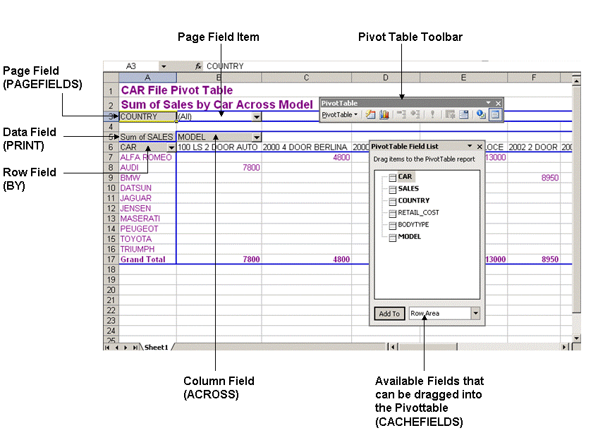
xEmbedding a WebFOCUS Report in an Excel 2000 Spreadsheet
Using an optional feature of
Excel called Microsoft Web Query, you can embed a WebFOCUS report
in a customized Excel spreadsheet that already contains styling, formulas,
and macros.
Microsoft Web Query uses a URL to embed external data or an HTML
page into the spreadsheet. Since you can easily construct a URL
that calls the WebFOCUS engine, you can use this URL as the source
of your query. Then, instead of following the typical reporting path
in which you execute a request from the browser and display the
output in an Excel spreadsheet that conforms to the formatting of
the report request, you can execute a request that returns HTML
from a query inside an existing Excel spreadsheet whose content
and layout you can control in Excel. Said another way, instead of
having WebFOCUS push the report into the spreadsheet, you can have
Excel pull the report into the spreadsheet. This "pull" technique
supports the delivery of real time data directly into your own customized
spreadsheets.
The process has two parts:
- Create the
WebFOCUS report, if you have not already done so.
- Designate the
area in your spreadsheet into which Microsoft Web Query will pull
the report, and provide Query with specifications for locating and
embedding it.
You must have a web browser installed on your PC to take advantage
of this technique.
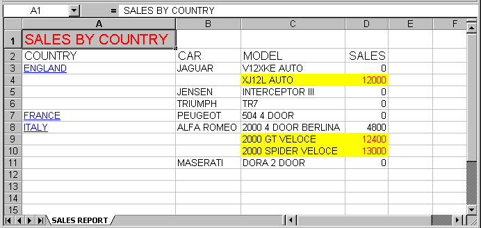
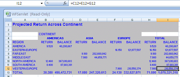
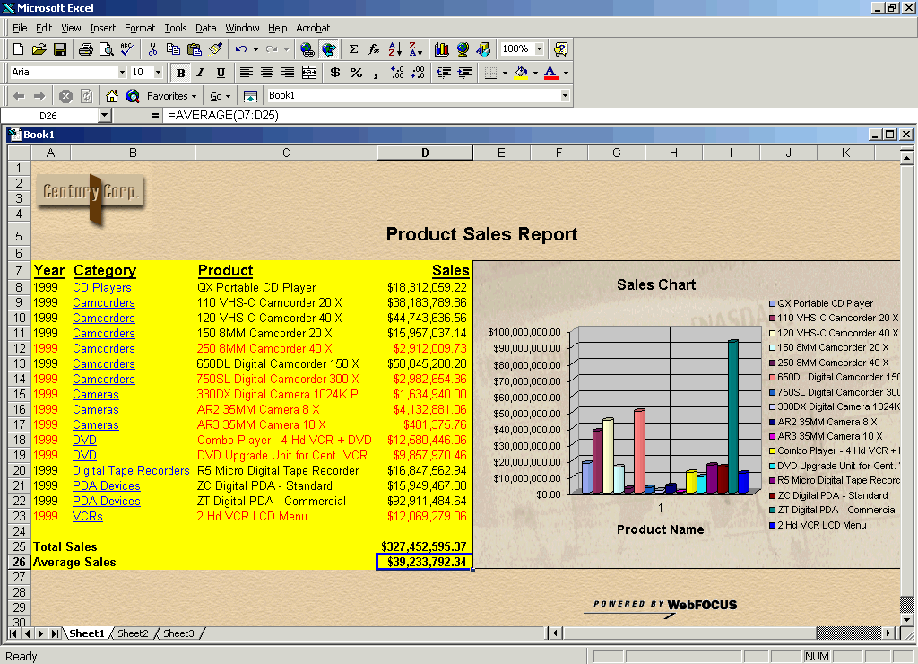
The following is a customized spreadsheet that was created using
this technique. Notice that it includes logos (images), a report,
formulas, and an Excel graph. There are two formulas added outside
of the query range that sum and average the data brought back by the
query. The report is generated as the result of a web query in the
area of the spreadsheet that has been designated to contain it.
The graph is also based on the results of this query. Each time
the query is refreshed, the formulas and the graph update as well.
After you understand the rudiments of this technique, you will
be able to adapt it to suit your preferred way of working with Excel.
For example, you can:
- Pull a WebFOCUS
report into an Excel spreadsheet that you have already customized
with logos (images), a report, formulas, or an Excel graph.
or
- Open a blank
spreadsheet, pull in a WebFOCUS report, and then customize the spreadsheet
as you like.
You can implement this technique, with some variations, in Excel
2000 and Excel 97. For illustrations, see Embedding a WebFOCUS Report in a Customized Excel 2000 Spreadsheet and Embedding a WebFOCUS Report in an Excel 97 Spreadsheet. For detail
on how to set up a web query in Excel 2000 or Excel 97, see your
Microsoft Excel documentation.
Note: Microsoft Web Query may not have been installed
by default. If you have not already installed it, you will be prompted
to install Web Query the first time you attempt to access the feature.
Just follow the install instructions provided.
Example: Embedding a WebFOCUS Report in a Customized Excel 2000 Spreadsheet
This
example creates the HTML report, then uses Web Query to set up the
customized spreadsheet to receive it.
Step 1: Create the WebFOCUS report
Create
and save the following request, webq.fex, which you will embed in
a customized Excel 200 spreadsheet: The numbers to the left of each
line of code correspond to annotations that follow the request.
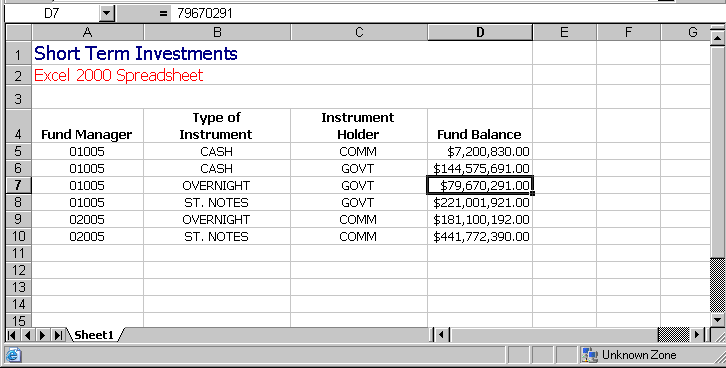
1.  TABLE FILE CENTORD
2.  SUM LINEPRICE AS 'Sales'
3.  BY PRODCAT
4.  BY PRODNAME
5.  ON TABLE PCHOLD FORMAT HTML
6.  ON TABLE SET HTMLCSS ON
7.  ON TABLE SET BYDISPLAY ON
8.  ON TABLE SET PAGE-NUM TOP
9.  ON TABLE SET STYLESHEET *
10. TYPE=REPORT, FONT=ARIAL, GRID=OFF, BACKCOLOR=YELLOW, $
11. TYPE=TITLE, STYLE=BOLD, $
12. TYPE=DATA, COLOR=RED, WHEN=LINEPRICE LT 15000000, $
13. ENDSTYLE
14. END
Line 1 identifies the sample data
source, CENTORD, which contains sales data for the Century corporation.
Lines 2-4 define
display and sorting requirements for the report.
Lines 5-6 define
the output format as HTML and turn on Cascading Style Sheets, a
feature that increases the efficiency and overall styling capabilities
of HTML.
Important: The report must be in HTML format
and not EXL2K. This is because Web Query imports fully formatted
HTML pages or individual HTML tables into a spreadsheet. Executing
an EXL2K request from a query will not return any data to the spreadsheet.
Line 7 sets
BYDISPLAY to ON. This optional setting ensures that repeated sort
values in the report are populated with data.
By default,
repeated sort values in vertical columns (or BY fields) are suppressed
in a WebFOCUS report, leaving blank fields in the report. This behavior
is not desirable for Excel reports, which are designed to work with
data that is repeated in every row to which it applies. A blank
column or row can produce misleading results when sorting data.
Line 8 turns
off page numbering and removes any extra lines generated above the
column titles.
Lines 9-12 specify styling attributes
for the report: background color, conditional styling, and some
other miscellaneous styling have been designated. Styling, including
drill-downs, carry over into Excel.
Step 2: Designate the area in the spreadsheet into which Web Query will pull the report
In
your spreadsheet, you designate the area where you want your WebFOCUS
report to be displayed. You can designate a cell and let Excel determine
how much space to allot to the report or you can specify a range
of cells to limit the placement. For some techniques that may help
you evaluate and control space requirements, see Tips for Populating Excel Spreadsheets With WebFOCUS Reports.
- Open a spreadsheet
and highlight the cell or range.
- From the Data
menu, select Get External Data, then select New
Web Query.
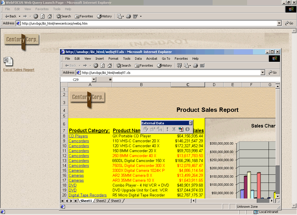
The New Web Query dialog box opens.

- In this dialog
box:
- Specify a URL
that points to the WebFOCUS server. The URL needs to be constructed
as a call to the WebFOCUS Servlet and contain any appropriate parameters
that need to be passed.
In the illustration, the code
http://servername/ibi_apps/WFServlet?IBIF_ex=webq
calls
the WebFOCUS Servlet and requests the procedure called webq.fex.
This is the report created in Step 1.
Keep in mind that you
may also need to pass a user ID and password to get to a secure
server. You must add parameters to the query manually. To do this,
save the query as an .iqy file and manually add parameters to the
URL request. For details, see How to Create a Web Query (IQY) File.
- Specify whether
the entire page or only the tables should be extracted from the requested
file. In this example, select the entire page.
Since WebFOCUS
HTML reports are generated using HTML tables, you can select either The
entire page or Only the tables.
(At the present time, you cannot identify individual tables in a WebFOCUS
HTML report.)
- Select Full
HTML formatting to ensure that all styling transfers
to the spreadsheet. This step is important if you want a styled
report to be carried over to Excel.
- Click OK.
- The Returning
External Data dialog box opens. Indicate the range of cells into
which you want the data to be returned in your spreadsheet.
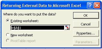
- Click the Properties button
in the Returning External Data dialog box. The External Data Range
Properties dialog box opens.

Name
the query and set its refresh behavior. For example, you can set
the query to automatically refresh every time the worksheet opens.
(Note that you can also set these properties after the initial execution.)
Click OK to
run the web query. The report is pulled into the area of the spreadsheet
that has been designated to contain it.
- Save the spreadsheet
with the embedded query. (Note that if you click the Save
Query button, the query information will be saved as
an .iqy file that you can use again with other worksheets.)
- After the query
is created and executed, you can customize your spreadsheet as much
as you like.
Note: You only need to run Web Query
once to embed a query in a worksheet. After it is executed, the
static data stays in the spreadsheet as a placeholder for the query. However,
as long as you are connected to your network, the internet, or whatever
other connection mechanism is in affect for your application, when
you open your local spreadsheet, WebFOCUS delivers the latest information
directly into your own customized spreadsheet. You can also click
the Refresh Data option at anytime to update
the information.
If you wish to delete a query, delete all
the query data in the spreadsheet.
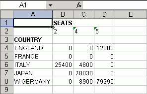
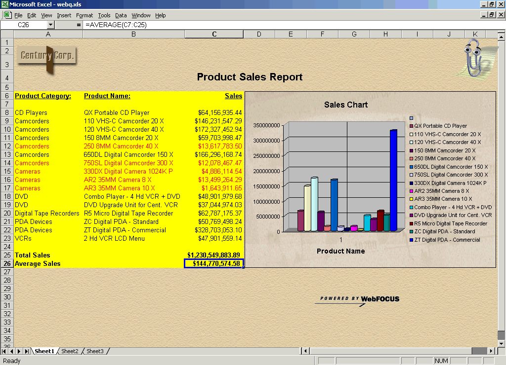
For an illustration of
a customized spreadsheet that contains the report created in step 1,
see Embedding a WebFOCUS Report in an Excel 2000 Spreadsheet. The spreadsheet
includes logos (images), a report, formulas, and an Excel graph.
The graph is also based on the results of this query. Each time
the query is refreshed, the formulas and the graph update as well.