Calculating Trends and Predicting Values With FORECAST
You can calculate trends in numeric data and predict values beyond the range of those stored in the data source by using the FORECAST feature. FORECAST can be used in a report or graph request.
The calculations you can make to identify trends and forecast values are:
- Simple moving average (FORECAST_MOVAVE). Calculates a series of arithmetic means using a specified number of values from a field. For details, see Using a Simple Moving Average.
- Exponential moving average. Calculates
a weighted average between the previously calculated value of the
average and the next data point. There are three methods for using
an exponential moving average:
- Single exponential smoothing (FORECAST_EXPAVE). Calculates an average that allows you to choose weights to apply to newer and older values. For details, see Using Single Exponential Smoothing.
- Double exponential smoothing (FORECAST_DOUBLEXP). Accounts for the tendency of data to either increase or decrease over time without repeating. For details, see Using Double Exponential Smoothing.
- Triple exponential smoothing (FORECAST_SEASONAL). Accounts for the tendency of data to repeat itself in intervals over time. For details, see Using Triple Exponential Smoothing.
- Linear regression analysis (FORECAST_LINEAR). Derives the coefficients of a straight line that best fits the data points and uses this linear equation to estimate values. For details, see Usage Notes for Creating Virtual Fields.
When predicting values in addition to calculating trends, FORECAST continues the same calculations beyond the data points by using the generated trend values as new data points. For the linear regression technique, the calculated regression equation is used to derive trend and predicted values.
FORECAST performs the calculations based on the data provided, but decisions about their use and reliability are the responsibility of the user. Therefore, the user is responsible for determining the reliability of the FORECAST predictions, based on the many factors that determine how accurate a prediction will be.
FORECAST Processing
|
Reference: |
You invoke FORECAST processing by including one of the FORECAST functions in a COMPUTE command. FORECAST performs the specified calculation for all the existing data points and then continues them to generate the number of predicted values that you request. The parameters needed for FORECAST include the field to use in the calculations, the number of predictions to generate, and whether to display the input field values or the calculated values on the report output for the rows that represent existing data points.
FORECAST operates on the lowest sort field in the request. This is either the last ACROSS field in the request or, if the request does not contain an ACROSS field, it is the last BY field. The FORECAST calculations start over when the highest-level sort field changes its value. In a request with multiple display commands, FORECAST operates on the last ACROSS field (or if there are no ACROSS fields, the last BY field) of the last display command. When using an ACROSS field with FORECAST, the display command must be SUM or COUNT.
Reference: Usage Notes for FORECAST
- The sort field used for FORECAST must be in a numeric or date format.
- When using simple moving average and exponential moving average methods, data values should be spaced evenly in order to get meaningful results.
- The use of column notation is not supported in the FORECAST expression. Column notation continues to be supported as before outside of this expression. The process of generating the FORECAST values creates extra columns that are not printed in the report output. The number and placement of these additional columns varies depending on the specific request.
- Missing values may lead to unexpected or unusable results and are not recommended for use with FORECAST_LINEAR.
- If you use the ESTRECORDS parameter to enable the external sort to better estimate the amount of sort work space needed, you must take into account that FORECAST with predictions creates additional records in the output.
- In a styled report,
you can assign specific attributes to values predicted by FORECAST with
the StyleSheet attribute WHEN=FORECAST. For example, to make the
predicted values display with the color red, use the following syntax
in the TABLE request:
ON TABLE SET STYLE *
TYPE=DATA,COLUMN=MYFORECASTSORTFIELD,WHEN=FORECAST,COLOR=RED,$
ENDSTYLE
Reference: FORECAST Limits
The following are not supported with a COMPUTE command that uses FORECAST:
- BY TOTAL command.
- MORE, MATCH, FOR, and OVER phrases.
FORECAST_MOVAVE: Using a Simple Moving Average
|
How to: |
A simple moving average is a series of arithmetic means calculated with a specified number of values from a field. Each new mean in the series is calculated by dropping the first value used in the prior calculation, and adding the next data value to the calculation.
Simple moving averages are sometimes used to analyze trends in stock prices over time. In this scenario, the average is calculated using a specified number of periods of stock prices. A disadvantage to this indicator is that because it drops the oldest values from the calculation as it moves on, it loses its memory over time. Also, mean values are distorted by extreme highs and lows, since this method gives equal weight to each point.
Predicted values beyond the range of the data values are calculated using a moving average that treats the calculated trend values as new data points.
The first complete moving average occurs at the nth data point because the calculation requires n values. This is called the lag. The moving average values for the lag rows are calculated as follows: the first value in the moving average column is equal to the first data value, the second value in the moving average column is the average of the first two data values, and so on until the nth row, at which point there are enough values to calculate the moving average with the number of values specified.
Syntax: How to Calculate a Simple Moving Average Column
FORECAST_MOVAVE(display, infield, interval,
 npredict, npoint1)
where:
- display
-
Keyword
Specifies which values to display for rows of output that represent existing data. Valid values are:
- INPUT_FIELD. This displays the original field values for rows that represent existing data.
- MODEL_DATA. This displays the calculated values for rows that represent existing data.
Note: You can show both types of output for any field by creating two independent COMPUTE commands in the same request, each with a different display option.
- infield
- Is any numeric field. It can be the same field as the result field, or a different field. It cannot be a date-time field or a numeric field with date display options.
- interval
- Is the increment to add to each sort field value (after
the last data point) to create the next value. This must be a positive
integer. To sort in descending order, use the BY HIGHEST phrase.
The result of adding this number to the sort field values
is converted to the same format as the sort field.
For date fields, the minimal component in the format determines how the number is interpreted. For example, if the format is YMD, MDY, or DMY, an interval value of 2 is interpreted as meaning two days. If the format is YM, the 2 is interpreted as meaning two months.
- npredict
- Is the number of predictions for FORECAST to calculate. It must
be an integer greater than or equal to zero. Zero indicates that
you do not want predictions, and is only supported with a non-recursive
FORECAST. For the SEASONAL method, npredict is the number of periods to
calculate. The number of points generated is:
nperiod * npredict
- npoint1
- Is the number of values to average for the MOVAVE method.
Example: Calculating a New Simple Moving Average Column
This request defines an integer value named PERIOD to use as the independent variable for the moving average. It predicts three periods of values beyond the range of the retrieved data. The MOVAVE column on the report output shows the calculated moving average numbers for existing data points.
DEFINE FILE GGSALES
SDATE/YYM = DATE;
SYEAR/Y = SDATE;
SMONTH/M = SDATE;
PERIOD/I2 = SMONTH;
END
TABLE FILE GGSALES
SUM UNITS DOLLARS
COMPUTE  MOVAVE/D10.1= FORECAST_MOVAVE(MODEL_DATA, DOLLARS,1,3,3);
BY CATEGORY BY PERIOD
WHERE SYEAR EQ 97 AND CATEGORY NE 'Gifts'
ON TABLE SET STYLE *
GRID=OFF,$
ENDSTYLE
END
The output is:
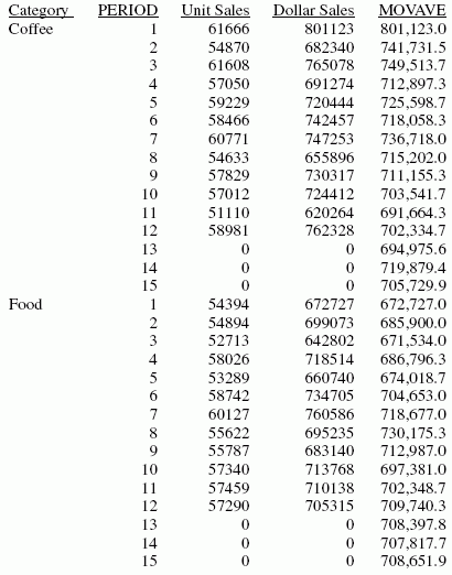
In the report, the number of values to use in the average is 3 and there are no UNITS or DOLLARS values for the generated PERIOD values.
Each average (MOVAVE value) is computed using DOLLARS values where they exist. The calculation of the moving average begins in the following way:
- The first MOVAVE value (801,123.0) is equal to the first DOLLARS value.
- The second MOVAVE value (741,731.5) is the mean of DOLLARS values one and two: (801,123 + 682,340) /2.
- The third MOVAVE value (749,513.7) is the mean of DOLLARS values one through three: (801,123 + 682,340 + 765,078) / 3.
- The fourth MOVAVE value (712,897.3) is the mean of DOLLARS values two through four: (682,340 + 765,078 + 691,274) /3.
For predicted values beyond the supplied values, the calculated MOVAVE values are used as new data points to continue the moving average. The predicted MOVAVE values (starting with 694,975.6 for PERIOD 13) are calculated using the previous MOVAVE values as new data points. For example, the first predicted value (694,975.6) is the average of the data points from periods 11 and 12 (620,264 and 762,328) and the moving average for period 12 (702,334.7). The calculation is: 694,975 = (620,264 + 762,328 + 702,334.7)/3.
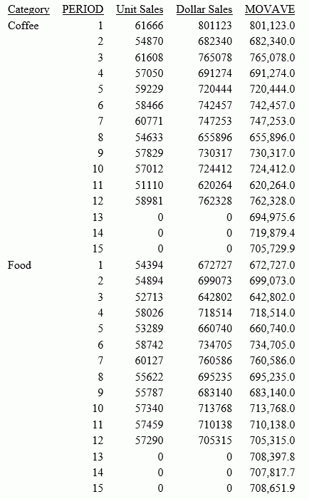
Example: Displaying Original Field Values in a Simple Moving Average Column
This request defines an integer value named PERIOD to use as the independent variable for the moving average. It predicts three periods of values beyond the range of the retrieved data. It uses the keyword INPUT_FIELD as the first argument in the FORECAST parameter list. The trend values do not display in the report. The actual data values for DOLLARS are followed by the predicted values in the report column.
DEFINE FILE GGSALES
SDATE/YYM = DATE;
SYEAR/Y = SDATE;
SMONTH/M = SDATE;
PERIOD/I2 = SMONTH;
END
TABLE FILE GGSALES
SUM UNITS DOLLARS
COMPUTE MOVAVE/D10.1 = FORECAST_MOVAVE(INPUT_FIELD,DOLLARS,1,3,3);
BY CATEGORY BY PERIOD
WHERE SYEAR EQ 97 AND CATEGORY NE 'Gifts'
ON TABLE SET STYLE *
GRID=OFF,$
ENDSTYLE
END
The output is shown in the following image:
FORECAST_EXPAVE: Using Single Exponential Smoothing
|
How to: |
The single exponential smoothing method calculates an average that allows you to choose weights to apply to newer and older values.
The following formula determines the weight given to the newest value.
k = 2/(1+n)
where:
- k
- Is the newest value.
- n
- Is an integer greater than one. Increasing n increases the weight assigned to the earlier observations (or data instances), as compared to the later ones.
The next calculation of the exponential moving average (EMA) value is derived by the following formula:
EMA = (EMA * (1-k)) + (datavalue * k)
This means that the newest value from the data source is multiplied by the factor k and the current moving average is multiplied by the factor (1-k). These quantities are then summed to generate the new EMA.
Note: When the data values are exhausted, the last data value in the sort group is used as the next data value.
Syntax: How to Calculate a Single Exponential Smoothing Column
FORECAST_EXPAVE(display, infield, interval,
 npredict, npoint1)
where:
- display
-
Keyword
Specifies which values to display for rows of output that represent existing data. Valid values are:
- INPUT_FIELD. This displays the original field values for rows that represent existing data.
- MODEL_DATA. This displays the calculated values for rows that represent existing data.
Note: You can show both types of output for any field by creating two independent COMPUTE commands in the same request, each with a different display option.
- infield
- Is any numeric field. It can be the same field as the result field, or a different field. It cannot be a date-time field or a numeric field with date display options.
- interval
- Is the increment to add to each sort field value (after
the last data point) to create the next value. This must be a positive
integer. To sort in descending order, use the BY HIGHEST phrase.
The result of adding this number to the sort field values
is converted to the same format as the sort field.
For date fields, the minimal component in the format determines how the number is interpreted. For example, if the format is YMD, MDY, or DMY, an interval value of 2 is interpreted as meaning two days. If the format is YM, the 2 is interpreted as meaning two months.
- npredict
- Is the number of predictions for FORECAST to calculate. It must be an integer greater than or equal to zero. Zero indicates that you do not want predictions, and is only supported with a non-recursive FORECAST.
- npoint1
- For
EXPAVE, this number is used to calculate
the weights for each component in the average. This value must be
a positive whole number. The weight, k, is calculated by the following
formula:
k=2/(1+npoint1)
Example: Calculating a Single Exponential Smoothing Column
The following defines an integer value named PERIOD to use as the independent variable for the moving average. It predicts three periods of values beyond the range of retrieved data.
DEFINE FILE GGSALES
SDATE/YYM = DATE;
SYEAR/Y = SDATE;
SMONTH/M = SDATE;
PERIOD/I2 = SMONTH;
END
TABLE FILE GGSALES
SUM UNITS DOLLARS
COMPUTE EXPAVE/D10.1= FORECAST_EXPAVE(MODEL_DATA,DOLLARS,1,3,3);
BY CATEGORY BY PERIOD
WHERE SYEAR EQ 97 AND CATEGORY NE 'Gifts'
ON TABLE SET STYLE *
GRID=OFF,$
ENDSTYLE
The output is shown in the following image:
Category     PERIOD  Unit Sales  Dollar Sales        EXPAVE
--------     ------  ----------  ------------        ------
Coffee            1       61666        801123     801,123.0
                  2       54870        682340     741,731.5
                  3       61608        765078     753,404.8
                  4       57050        691274     722,339.4
                  5       59229        720444     721,391.7
                  6       58466        742457     731,924.3
                  7       60771        747253     739,588.7
                  8       54633        655896     697,742.3
                  9       57829        730317     714,029.7
                 10       57012        724412     719,220.8
                 11       51110        620264     669,742.4
                 12       58981        762328     716,035.2
                 13           0             0     739,181.6
                 14           0             0     750,754.8
                 15           0             0     756,541.4
Food              1       54394        672727     672,727.0
                  2       54894        699073     685,900.0
                  3       52713        642802     664,351.0
                  4       58026        718514     691,432.5
                  5       53289        660740     676,086.3
                  6       58742        734705     705,395.6
                  7       60127        760586     732,990.8
                  8       55622        695235     714,112.9
                  9       55787        683140     698,626.5
                 10       57340        713768     706,197.2
                 11       57459        710138     708,167.6
                 12       57290        705315     706,741.3
                 13           0             0     706,028.2
                 14           0             0     705,671.6
                 15           0             0     705,493.3
In the report, three predicted values of EXPAVE are calculated within each value of CATEGORY. For values outside the range of the data, new PERIOD values are generated by adding the interval value (1) to the prior PERIOD value.
Each average (EXPAVE value) is computed using DOLLARS values where they exist. The calculation of the moving average begins in the following way:
- The first EXPAVE value (801,123.0) is the same as the first DOLLARS value.
- The second EXPAVE
value (741,731.5) is calculated as follows. Note that because of
rounding and the number of decimal places used, the value derived
in this sample calculation varies slightly from the one displayed
in the report output:
n=3 (number used to calculate weights)
k = 2/(1+n) = 2/4 = 0.5
EXPAVE = (EXPAVE*(1-k))+(new-DOLLARS*k) = (801123*0.5) + (682340*0.50) = 400561.5 + 341170 = 741731.5
- The third EXPAVE
value (753,404.8) is calculated as follows:
EXPAVE = (EXPAVE*(1-k))+(new-DOLLARS*k) = (741731.5*0.5)+(765078*0.50) = 370865.75 + 382539 = 753404.75
FORECAST_DOUBLEXP: Using Double Exponential Smoothing
|
How to: |
Double exponential smoothing produces an exponential moving average that takes into account the tendency of data to either increase or decrease over time without repeating. This is accomplished by using two equations with two constants.
- The first equation
accounts for the current time period and is a weighted average of
the current data value and the prior average, with an added component
(b) that represents the trend for the previous period. The weight
constant is k:
DOUBLEXP(t) = k * datavalue(t) + (1-k) * ((DOUBLEXP(t-1) + b(t-1))
- The second equation
is the calculated trend value, and is a weighted average of the
difference between the current and previous average and the trend
for the previous time period. b(t) represents the average
trend. The weight constant is g:
b(t) = g * (DOUBLEXP(t)-DOUBLEXP(t-1)) + (1 - g) * (b(t-1))
These two equations are solved to derive the smoothed average. The first smoothed average is set to the first data value. The first trend component is set to zero. For choosing the two constants, the best results are usually obtained by minimizing the mean-squared error (MSE) between the data values and the calculated averages. You may need to use nonlinear optimization techniques to find the optimal constants.
The equation used for forecasting beyond the data points with double exponential smoothing is
forecast(t+m) = DOUBLEXP(t) + m * b(t)
where:
- m
- Is the number of time periods ahead for the forecast.
Syntax: How to Calculate a Double Exponential Smoothing Column
FORECAST_DOUBLEXP(display, infield,
interval, npredict, npoint1, npoint2)
where:
- display
-
Keyword
Specifies which values to display for rows of output that represent existing data. Valid values are:
- INPUT_FIELD. This displays the original field values for rows that represent existing data.
- MODEL_DATA. This displays the calculated values for rows that represent existing data.
Note: You can show both types of output for any field by creating two independent COMPUTE commands in the same request, each with a different display option.
- infield
- Is any numeric field. It can be the same field as the result field, or a different field. It cannot be a date-time field or a numeric field with date display options.
- interval
- Is the increment to add to each sort field value (after
the last data point) to create the next value. This must be a positive
integer. To sort in descending order, use the BY HIGHEST phrase.
The result of adding this number to the sort field values
is converted to the same format as the sort field.
For date fields, the minimal component in the format determines how the number is interpreted. For example, if the format is YMD, MDY, or DMY, an interval value of 2 is interpreted as meaning two days. If the format is YM, the 2 is interpreted as meaning two months.
- npredict
- Is the number of predictions for FORECAST to calculate. It must be an integer greater than or equal to zero. Zero indicates that you do not want predictions, and is only supported with a non-recursive FORECAST.
- nperiod
- For the SEASONAL method, it is a positive whole number that specifies the number of data points in a period.
- npoint1
- For
DOUBLEXP, this number is used to calculate
the weights for each component in the average. This value must be
a positive whole number. The weight, k, is calculated by the following
formula:
k=2/(1+npoint1)
- npoint2
- For DOUBLEXP, this positive whole number is used
to calculate the weights for each term in the trend. The weight,
g, is calculated by the following formula:
g=2/(1+npoint2)
Example: Calculating a Double Exponential Smoothing Column
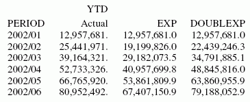
The following sums the ACTUAL_YTD field of the CENTSTMT data source by period, and calculates a single exponential and double exponential moving average. The report columns show the calculated values for existing data points.
TABLE FILE CENTSTMT
SUM ACTUAL_YTD
COMPUTE EXP/D15.1 = FORECAST_EXPAVE(MODEL_DATA,ACTUAL_YTD,1,0,3);
DOUBLEXP/D15.1 = FORECAST_DOUBLEXP(MODEL_DATA,ACTUAL_YTD,1,0,3,3);
BY PERIOD
WHERE GL_ACCOUNT LIKE '3%%%'
ON TABLE SET STYLE *
GRID=OFF,$
END
The output is shown in the following image:
FORECAST_SEASONAL: Using Triple Exponential Smoothing
|
How to: |
Triple exponential smoothing produces an exponential moving average that takes into account the tendency of data to repeat itself in intervals over time. For example, sales data that is growing and in which 25% of sales always occur during December contains both trend and seasonality. Triple exponential smoothing takes both the trend and seasonality into account by using three equations with three constants.
For triple exponential smoothing you, need to know the number of data points in each time period (designated as L in the following equations). To account for the seasonality, a seasonal index is calculated. The data is divided by the prior season index and then used in calculating the smoothed average.
- The first equation
accounts for the current time period, and is a weighted average
of the current data value divided by the seasonal factor and the
prior average adjusted for the trend for the previous period. The
weight constant is k:
SEASONAL(t) = k * (datavalue(t)/I(t-L)) + (1-k) * (SEASONAL(t-1) + b(t-1))
- The second equation
is the calculated trend value, and is a weighted average of the
difference between the current and previous average and the trend
for the previous time period. b(t) represents the average
trend. The weight constant is g:
b(t) = g * (SEASONAL(t)-SEASONAL(t-1)) + (1-g) * (b(t-1))
- The third equation
is the calculated seasonal index, and is a weighted average of the
current data value divided by the current average and the seasonal
index for the previous season. I(t) represents the average
seasonal coefficient. The weight constant is p:
I(t) = p * (datavalue(t)/SEASONAL(t)) + (1 - p) * I(t-L)
These equations are solved to derive the triple smoothed average. The first smoothed average is set to the first data value. Initial values for the seasonality factors are calculated based on the maximum number of full periods of data in the data source, while the initial trend is calculated based on two periods of data. These values are calculated with the following steps:
- The initial trend
factor is calculated by the following formula:
b(0) = (1/L) ((y(L+1)-y(1))/L + (y(L+2)-y(2))/L + ... + (y(2L) -
y(L))/L )
- The calculation of
the initial seasonality factor is based on the average of the data values
within each period, A(j) (1<=j<=N):
A(j) = ( y((j-1)L+1) + y((j-1)L+2) + ... + y(jL) ) / L
- Then, the initial
periodicity factor is given by the following formula, where N is
the number of full periods available in the data, L is the number
of points per period and n is a point within the period (1<=
n <= L):
I(n) = ( y(n)/A(1) + y(L+n)/A(2) + ... + y((N-1)L+n)/A(N) ) / N
The three constants must be chosen carefully. The best results are usually obtained by choosing the constants to minimize the mean-squared error (MSE) between the data values and the calculated averages. Varying the values of npoint1 and npoint2 affect the results, and some values may produce a better approximation. To search for a better approximation, you may want to find values that minimize the MSE.
The equation used to forecast beyond the last data point with triple exponential smoothing is:
forecast(t+m) = (SEASONAL(t) + m * b(t)) / I(t-L+MOD(m/L))
where:
- m
- Is the number of periods ahead for the forecast.
Syntax: How to Calculate a Triple Exponential Smoothing Column
FORECAST_SEASONAL(display, infield,
interval, npredict, nperiod, npoint1, npoint2, npoint3)
where:
- display
-
Keyword
Specifies which values to display for rows of output that represent existing data. Valid values are:
- INPUT_FIELD. This displays the original field values for rows that represent existing data.
- MODEL_DATA. This displays the calculated values for rows that represent existing data.
Note: You can show both types of output for any field by creating two independent COMPUTE commands in the same request, each with a different display option.
- infield
- Is any numeric field. It can be the same field as the result field, or a different field. It cannot be a date-time field or a numeric field with date display options.
- interval
- Is the increment to add to each sort field value (after
the last data point) to create the next value. This must be a positive
integer. To sort in descending order, use the BY HIGHEST phrase.
The result of adding this number to the sort field values
is converted to the same format as the sort field.
For date fields, the minimal component in the format determines how the number is interpreted. For example, if the format is YMD, MDY, or DMY, an interval value of 2 is interpreted as meaning two days. If the format is YM, the 2 is interpreted as meaning two months.
- npredict
- Is the number of predictions for FORECAST to calculate. It must
be an integer greater than or equal to zero. Zero indicates that
you do not want predictions, and is only supported with a non-recursive
FORECAST. For the SEASONAL method, npredict is the number of periods to
calculate. The number of points generated is:
nperiod * npredict
- nperiod
- For the SEASONAL method, is a positive whole number that specifies the number of data points in a period.
- npoint1
- For
SEASONAL, this number is used to calculate
the weights for each component in the average. This value must be
a positive whole number. The weight, k, is calculated by the following
formula:
k=2/(1+npoint1)
- npoint2
- For SEASONAL, this positive whole number is used
to calculate the weights for each term in the trend. The weight,
g, is calculated by the following formula:
g=2/(1+npoint2)
- npoint3
- For SEASONAL, this positive whole number is used to calculate
the weights for each term in the seasonal adjustment. The weight,
p, is calculated by the following formula:
p=2/(1+npoint3)
Example: Calculating a Triple Exponential Smoothing Column
In the following, the data has seasonality but no trend. Therefore, npoint2 is set high (1000) to make the trend factor negligible in the calculation:
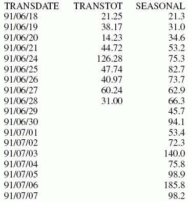
TABLE FILE VIDEOTRK
SUM TRANSTOT
COMPUTE SEASONAL/D10.1 = FORECAST_SEASONAL(MODEL_DATA,TRANSTOT,1,3,3,3,1000,1);
BY TRANSDATE
WHERE TRANSDATE NE '19910617'
ON TABLE SET STYLE *
GRID=OFF,$
ENDSTYLE
END
In the output, npredict is 3. Therefore, three periods (nine points, nperiod * npredict) are generated.
FORECAST_LINEAR: Using a Linear Regression Equation
|
How to: |
The linear regression equation estimates values by assuming that the dependent variable (the new calculated values) and the independent variable (the sort field values) are related by a function that represents a straight line:
y = mx + b
where:
- y
- Is the dependent variable.
- x
- Is the independent variable.
- m
- Is the slope of the line.
- b
- Is the y-intercept.
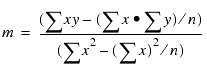
FORECAST_LINEAR uses a technique called Ordinary Least Squares to calculate values for m and b that minimize the sum of the squared differences between the data and the resulting line.
The following formulas show how m and b are calculated.
where:
- n
- Is the number of data points.
- y
- Is the data values (dependent variables).
- x
- Is the sort field values (independent variables).
Trend values, as well as predicted values, are calculated using the regression line equation.
Syntax: How to Calculate a Linear Regression Column
FORECAST_LINEAR(display, infield, interval,
 npredict)
where:
- display
-
Keyword
Specifies which values to display for rows of output that represent existing data. Valid values are:
- INPUT_FIELD. This displays the original field values for rows that represent existing data.
- MODEL_DATA. This displays the calculated values for rows that represent existing data.
Note: You can show both types of output for any field by creating two independent COMPUTE commands in the same request, each with a different display option.
- infield
- Is any numeric field. It can be the same field as the result field, or a different field. It cannot be a date-time field or a numeric field with date display options.
- interval
- Is the increment to add to each sort field value (after
the last data point) to create the next value. This must be a positive
integer. To sort in descending order, use the BY HIGHEST phrase.
The result of adding this number to the sort field values
is converted to the same format as the sort field.
For date fields, the minimal component in the format determines how the number is interpreted. For example, if the format is YMD, MDY, or DMY, an interval value of 2 is interpreted as meaning two days. If the format is YM, the 2 is interpreted as meaning two months.
- npredict
- Is the number of predictions for FORECAST to calculate. It must be an integer greater than or equal to zero. Zero indicates that you do not want predictions, and is only supported with a non-recursive FORECAST.
Example: Calculating a New Linear Regression Field
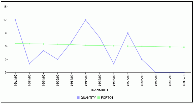
The following request calculates a regression line using the VIDEOTRK data source of QUANTITY by TRANSDATE. The interval is one day, and three predicted values are calculated.
TABLE FILE VIDEOTRK
SUM QUANTITY
COMPUTE FORTOT=FORECAST_LINEAR(MODEL_DATA,QUANTITY,1,3);
BY TRANSDATE
ON TABLE SET PAGE NOLEAD
ON TABLE SET STYLE *
GRID=OFF,$
ENDSTYLE
END
The output is shown in the following image:
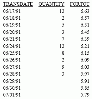
Note:
- Three predicted values of FORTOT are calculated. For values outside the range of the data, new TRANSDATE values are generated by adding the interval value (1) to the prior TRANSDATE value.
- There are no QUANTITY values for the generated FORTOT values.
- Each FORTOT value
is computed using a regression line, calculated using all of the actual
data values for QUANTITY.
TRANSDATE is the independent variable (x) and QUANTITY is the dependent variable (y). The equation is used to calculate QUANTITY FORECAST trend and predicted values.
The following version of the request charts the data values and the regression line.
GRAPH FILE VIDEOTRK
SUM QUANTITY
COMPUTE FORTOT=FORECAST_LINEAR(MODEL_DATA,QUANTITY,1,3);
BY TRANSDATE
ON GRAPH HOLD FORMAT JSCHART
ON GRAPH SET LOOKGRAPH VLINE
END
The output is shown in the following image.
Distinguishing Data Rows From Predicted Rows
To make the report output easier to interpret, you can create a field that indicates whether the FORECAST value in each row is a predicted value. To do this, define a virtual field whose value is a constant other than zero. Rows in the report output that represent actual records in the data source will appear with a value that is not zero. Rows that represent predicted values will display zero. You can also propagate this field to a HOLD file.
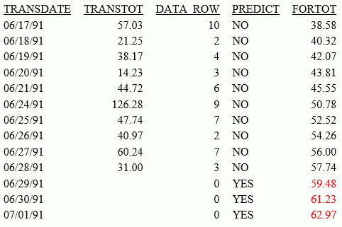
Example: Distinguishing Data Rows From Predicted Rows
In the following example, the DATA_ROW virtual field has the value 1 for each row in the data source. It has the value zero for the predicted rows. The PREDICT field is calculated as YES for predicted rows, and NO for rows containing data. In addition, the StyleSheet attribute WHEN=FORECAST is used to display the predicted values for the FORTOT field in red.
DEFINE FILE VIDEOTRK
DATA_ROW/I1 = 1;
END
TABLE FILE VIDEOTRK
SUM TRANSTOT DATA_ROW
COMPUTE
PREDICT/A3 = IF DATA_ROW NE 0 THEN 'NO' ELSE 'YES' ;
FORTOT/D12.2=FORECAST_LINEAR(MODEL_DATA,TRANSTOT,1,3);
BY TRANSDATE
ON TABLE SET PAGE NOLEAD
ON TABLE SET STYLE *
GRID=OFF,$
TYPE=DATA, COLUMN=FORTOT, WHEN=FORECAST, COLOR=RED,$
ENDSTYLE
END
The output is shown in the following image: