Assigning XLSX Format to Your Report Output
XLSX (Excel 2007/2010) format generates fully styled reports in Excel 2007/2010 binary display format. The FOCUS procedure generates a new workbook containing a single worksheet with the report output containing your defined report elements (headings and subtotals), as well as StyleSheet syntax (such as conditional styling and drilldowns):
- XLSX format accurately displays formatted numeric, character and date formats.
- Within each generated worksheet, the columns in the report are automatically sized to fit the largest value in the column. FOCUS calculates the width of each data column based on the font and size requirement of all cells in that column using font metrics developed for other styled formats, including PDF and DHTML. Calculations are based on the data and title elements of the report. Heading and footing elements are not used in the sizing calculation and will be sized based on the data column requirements.
- Tab names within the workbook can be customized to provide better descriptions of the worksheet content using the TITLETEXT StyleSheet attribute described in How to Name Worksheets.
- By default, leading, internal, and trailing blanks are compressed in cells within the worksheet.
- An Excel 2007/2010 worksheet can contain 1,048,576 rows by 16,384 columns. FOCUS will generate worksheets larger than these defined limits, but Excel 2007/2010 will have difficulty opening the resulting workbook, and the data that exceeds the Excel 2007/2010 limits will be truncated.
Overview of XLSX Format
|
How to: |
|
Reference: |
In order to open Excel 2007/2010 workbooks generated in either the browser or the Excel application, you must have Excel 2007 or greater installed on the desktop.
Excel 2000 and Excel 2003 can be updated to read Excel 2007 or 2010 workbooks using the Microsoft Office Compatibility Pack available from the Microsoft download site (http://www.microsoft.com/downloads/en/default.aspx).
Reference: Building the XLSX Workbook File
Microsoft changed the format and structure of the Excel workbook in Excel 2007. The new .xlsx file is a binary compilation of a group of XML files. Generating this new file format using FOCUS is a two step process that consists of generating the XML files containing the report output and zipping the XML documents into the binary .xlsx format.
The zipping process requires code included in the webfocus.war file of the WebFOCUS client, which is deployed as the ibi_apps context root on an application server such as Tomcat.
You must have an installed version of the WebFOCUS Client so that ibi_apps is deployed. The application server must be running when you issue the HOLD FORMAT XLSX command in your report request. The WebFOCUS Client does not have to be running. Your request must point to the URL where ibi_apps is deployed using the SET EXCELSERVURL command:
SET EXCELSERVURL = http://servername:8080/ibi_apps
where:
- servername
-
Is the name of the machine where the application server is running.
- 8080
-
Is the default port used by the WebFOCUS Client to communicate with the application server.
After the XLSX output file is generated, you must FTP it to your PC in binary mode.
Note: This setting is also required for generating PPTX output files.
Syntax: How to Generate an Excel 2007 or 2010 Workbook
You can specify that a report should be saved to an Excel 2007/2010 workbook, displayed in the browser, or displayed in the Excel 2007/2010 application.
ON TABLE HOLD AS name FORMAT XLSX
where:
- name
-
Specifies a file name for the generated workbook.
Formatting Values Within Cells in XLSX Report Output
FOCUS formats defined in Master Files or within a FOCEXEC will be represented in the resulting cells in an Excel 2007 or 2010 worksheet. Where possible, the FOCUS formats are translated to custom Excel formats and applied to values passed as raw data. Each data value passed to a cell in Excel 2007/2010 is defined with a value and a format mask pair. The data format is associated with the cell rather than embedded in the value. This technique provides enhanced support for editing worksheets generated by FOCUS. New values entered into existing cells will retain the cell formats and continue to display in the style defined for the column within the report.
The following type of data can be passed to Excel 2007/2010:
- Numeric. Where corresponding Excel format masks can be defined, numeric values are passed as raw values with associated format masks. In instances where an equivalent format mask cannot be defined, the numeric value is passed as a text string.
- Alphanumeric. Alphanumeric formats are passed to Excel 2007/2010 as text strings, with General format defined. By default, General format presents all text fields as left justified. Alignment and other styling attributes can be applied to these cells to override the default.
- Date formats. Data that contain sufficient elements to define a valid Excel date format are passed as raw date values with the FOCUS data formats translated to Excel date format masks. In FOCUS formats that do not contain sufficient information to create valid Excel date values, the dates are converted to text strings.
- Date-Time formats. Date-time values are passed as raw date-time values with FOCUS formats translated to Excel date-time format masks using Custom formats.
- Text. Text values are passed as strings with General Format defined (as with alphanumeric data).
Note: This behavior is a change from EXL2K format, where cells containing dates and more complex numeric formats were passed as formatted text.
Displaying Formatted Numeric Values in XLSX Report Output
Each numeric FOCUS format is translated to a custom numeric Excel format. The numeric value is displayed in the Excel formula bar for the selected cell. Within the actual cell, the value with the format mask applied displays.
The FOCUS formats for the following numeric data types are translated into Excel 2007/2010 format masks supporting full editing within the resulting workbook:
- Data types: E, F, D , I, P.
- Comma edit option (C).
- Zero suppression (S).
- Leading zero (L).
- Floating currency symbol (M).
- Comma Suppression (c).
- Right-side minus sign (-).
- Credit negative (CR).
- Bracket negative (B).
- Fixed extended currency symbol (!d, !e, !l, !y).
- Floating extended currency symbol (!D, !E, !L, !Y).
- Percent (%).
Example: Passing Numeric Formats to XLSX Report Output
In the following example, the DOLLARS field is assigned different numeric formats to demonstrate different available options. The column titles have been edited to display the FOCUS format options that have been applied:
TABLE FILE GGSALES
SUM DOLLARS/D12.2 AS 'D12.2'
    DOLLARS/D12C  AS 'D12C'
    DOLLARS/D12CM AS 'D12CM'
BY REGION
BY CATEGORY
ON TABLE HOLD FORMAT XLSX
ON TABLE SET BYDISPLAY ON
END
In the resulting worksheet, notice that cell C2 containing the DOLLAR value for Midwest Coffee presents the value with the FOCUS format D12.2, which presents the comma and two decimal places. On the formula bar, the actual value is presented without any formatting. Examine each of the DOLLAR values in each row to see that the value as displayed in the formula bar remains the same, and only the display values presented in each cell change.
Also notice that with SET BYDISPLAY ON, the BY field values are repeated for every row on the worksheet. This creates fully qualified data rows that can be used with various data sorting, filtering, and table features in Excel without losing valuable information. This setting is recommended as a best practice for all worksheets:
The following example uses Fixed Dollar (N) format, as well as multiple combined format options. Each FOCUS format option is translated to the appropriate Excel 2007/2010 format mask and applied to the cell value:
TABLE FILE GGSALES
SUM BUDDOLLARS/D12N
    DOLLARS/D12M
COMPUTE OVERBUDGET/D12BMc=BUDDOLLARS-DOLLARS; AS 'Over Budget'
BY REGION
BY CATEGORY
ON TABLE HOLD FORMAT XLSX
ON TABLE SET BYDISPLAY ON
END
Notice the fixed numeric format defined for the BUDDOLLARS column (Column C) presents the local currency symbol in a fixed position within each cell, regardless of the size of the data value. On the formula bar, the values in the Over Budget calculated field is passed as a negative value where appropriate. In the actual cells, the bracketed styling is applied to the negative values as part of the custom Excel 2007/2010 format mask:
Using Numeric Formats in Report Headings and Footings
By default, headings and footings are passed to Excel as a single character string. Spot markers are not supported for positioning within each line. Numeric fields and dates passed in headings and footings are passed as text strings within the overall heading or footing contents.
To display numeric fields and dates within headings and footings as numeric or date values, use HEADALIGN=BODY in the StyleSheet to define each of the items in the heading as an individual cell. Each cell containing numeric or date values will then be passed as the appropriate value with the associated format mask.
For information about the HEADALIGN attribute, see Aligning a Heading or Footing Element in an HTML, EXL07, EXL2K, or PDF Report.
Using Numeric Format Punctuation in Headings and Footings
For data columns, all currency formats are translated using the Excel 2007/2010 format masks that use the punctuation rules defined by the regional settings of the desktop.
In languages that use Continental Decimal Notation, the currency definitions designate that a comma is used as the decimal separator, and a period is used as the thousands separator, so D12.2CM may present the value as $ 9.999,99 rather than the English (United States) value $ 9,999.99. In headings and footings, you can designate that punctuation should be converted to Continental Decimal notation by issuing the SET CDN=ON command. With this setting in effect, the data embedded within heading and footing text strings will be formatted using the converted punctuation. Specify HEADALIGN=BODY to delineate items as individual cells and to retain the numeric formatting within the field which will follow the same rules as the report data within the data columns.
Passing Dates to XLSX Report Output
Most translated and smart dates can be sent to Excel 2007/2010 as standard date values with format masks, enabling Excel to use them in functions, formulas, and sort sequences.
Example: Translating FOCUS Dates to Excel 2007/2010 Dates
The following request against the GGSALES data source creates the date January 1, 2010 and converts it to four date formats with translated text:
DEFINE FILE GGSALES
NEWDATE/MDYY = '01/01/2010';
WRMtrDY/WRMtrDY = NEWDATE;
wDMTY/wDMTY= NEWDATE;
wrDMTRY/wrDMTRY= NEWDATE;
wrYMtrD/wrYMtrD= NEWDATE;
END
TABLE FILE GGSALES
SUM DATE NOPRINT
NEWDATE WRMtrDY wDMTY wrDMTRY wrYMtrD
ON TABLE HOLD FORMAT XLSX
END
The following table shows how the dates should appear:
|
FOCUS Format |
XLSX Displays |
XLSX Value |
|---|---|---|
|
WRMtrDY |
Friday, January 1 10 |
1/1/2010 |
|
wDMTY |
Fri, 1 Jan 10 |
1/1/2010 |
|
wrDMTRY |
Friday, 1 January 1 |
1/1/2010 |
|
wrYMtrD |
Friday, 10 January 1 |
1/1/2010 |
In Excel 2007/2010, all of the cells have a date value with format masks, and all month and day names are in mixed-case, regardless of how the case has been specified in the FOCUS format. The output is:
Passing Dates Without a Day Component
Date formats that do not specify the day value explicitly are defined as the date value of the first day of the month. Therefore, the value placed in the cell may be different from the day component value in the source data field and may produce unexpected results when used for sorting or date calculations in an Excel formula.
The following table shows how FOCUS date formats are represented in XLSX. The table shows how the value is preserved in the cell and how the display is generated using the format mask that corresponds to the FOCUS date format.
DATEFLD/MDYY = '01/02/2010'
|
FOCUS Format |
XLSX Displays: |
XLSX Value |
|---|---|---|
|
DMYY |
02/01/2010 |
1/2/2010 |
|
MY |
01/10 |
1/1/2010 |
|
MTY |
Jan, 10 |
1/1/2010 |
|
MTDY |
Jan 2, 10 |
1/2/2010 |
Example: Passing FOCUS Dates With and Without a Day Component to XLSX Report Output
The following request against the GGSALES data source creates the date January 2, 2010 and passes it to Excel 2007/2010 with formats MDYY, DMYY, MY, and MTDY:
DEFINE FILE GGSALES
NEWDATE/MDYY = '01/02/2010';
END
TABLE FILE GGSALES
SUM DATE NOPRINT
NEWDATE AS 'MDYY' NEWDATE/DMYY AS 'DMYY' NEWDATE/MY AS 'MY'
        NEWDATE/MTY AS 'MTY' NEWDATE/MTDY AS 'MTDY'
ON TABLE HOLD FORMAT XLSX
END
Columns D and E have actual date values with format masks, displayed by Excel 2007/2010 in mixed-case. Since the MTY format does not have a day component, the date value stored is the first of January 2010 (1/1/2010), not the second of January 2010 (1/2/2010):
Passing Date Components for Use in Excel Formulas
Dates formatted as individual components (for example, D, Y, M, W) are passed to Excel as numeric values that can be used as parameters to Excel date functions. The values are passed as general format that are recognized by Excel as numbers.
Example: Passing Numeric Date Components to XLSX Report Output
The following request against the GGSALES data source creates the date January 1, 2010 and extracts numeric date components, passing them to Excel 2007/2010:
DEFINE FILE GGSALES
NEWDATE/MDYY = '01/01/2010';
D/D= NEWDATE;
Y/Y = NEWDATE;
W/W=NEWDATE;
w/w=NEWDATE;
M/M = NEWDATE;
YY/YY = NEWDATE;
END
TABLE FILE GGSALES
SUM DATE NOPRINT
NEWDATE D Y W w M YY
ON TABLE HOLD FORMAT XLSX
END
The output is:
Passing Quarter Formats
Date formats that contain a Quarter component are always passed to Excel as text strings since Excel does not support Quarter formats.
Example: Passing Dates With a Quarter Component to Excel 2007
The following request against the GGSALES data source creates the date January 1, 2010 and converts it to date formats that contain a Quarter component:
DEFINE FILE GGSALES
NEWDATE/MDYY = '01/01/2010';
Q/Q= NEWDATE;
QY/QY = NEWDATE;
YBQ/YBQ=NEWDATE;
END
TABLE FILE GGSALES
SUM DATE NOPRINT
NEWDATE Q QY YBQ
ON TABLE HOLD FORMAT XLSX
END
In Excel 2007 or 2010, the cells containing dates with Quarter components have General format. To see this, open the Format Cells dialog box.
The output is:
Passing Date Components Defined as Translated Text
|
Reference: |
Date formats that do not contain sufficient information to present a valid date result in Excel are not translated to a value, including formats that do not contain year and/or month information. These dates will be sent to Excel as text. In the absence of complete information, the year defaults to the current year, so the value sent would be incorrect if this type of format was passed as a date value. The following formats will not be sent as values:
- MT, MTR, Mt, Mtr
- W, w, WR, wr
When date formats are passed to Excel 2007/2010 with format masks, all month and day names are in mixed-case, regardless of how the case has been specified in the FOCUS format. However, since the values in this example are always sent as text, the casing defined in the FOCUS format is applied in the resulting cell.
Example: Passing Date Components Defined as Translated Text to XLSX Report Output
The following request against the GGSALES data source creates the date January 1, 2010 and converts it to date formats that are defined as either month name or day name:
DEFINE FILE GGSALES
NEWDATE/MDYY = '01/01/2010';
MT/MT= NEWDATE;
MTR/MTR= NEWDATE;
Mtr/Mtr = NEWDATE;
WR/WR = NEWDATE;
wr/wr = NEWDATE;
END
TABLE FILE GGSALES
SUM DATE NOPRINT
NEWDATE MT MTR Mtr WR wr
ON TABLE HOLD FORMAT XLSX
END
In Excel 2007 or 2010, the cells containing the days have General format. To see this, open the Format Cells dialog box.
The output is:
![]()
Reference: Usage Notes for Date Values in XLSX Report Output
- The following date formats are not supported in XLSX. They will
translate into Excel General format and possibly produce unpredictable
results:
- JUL, YYJUL, and I2MT.
- Dates stored as a packed or alphanumeric field with date display options.
- Excel only supports mixed-case, not all uppercase or all lowercase for text dates. All FOCUS date formats containing text present in XLSX as mixed-case, regardless of the casing parameters defined in the FOCUS format. For example, MTRDY will generate the date string JANUARY 2, 10 in standard FOCUS, but when sent to XLSX as a date value, it will be presented as January 2, 10.
Passing Date-Time to XLSX
Most FOCUS date-time formats can be sent to XLSX as standard date/time values with format masks, enabling Excel to use them in functions, formulas, and sort sequences.
As with the Date formats, Excel only supports mixed-case to date-time fields, so if the date-time format contains text and is supported by Excel, the text will be in mixed-case, regardless of the casing defined within the FOCUS format.
Example: Passing Date-Time to XLSX
The following request shows an example against the GGSALES data source.
DEFINE FILE GGSALES
DT1/HYYMDm WITH REGION = DT(20100506 16:17:01.993876);
DPT1/HDMTYYm = DT1;
ALPHA_DATE1/A30 = HCNVRT(DT1,'(HYYMDm)',30,'A30');
END
TABLE FILE GGSALES
PRINT
ALPHA_DATE1
DT1 AS 'HYYMDm'
DPT1 AS 'HDMTYYm'
DT1/HdMTYYBS   AS 'HdMTYYBS'
DT1/HdMTYYBs   AS 'HdMTYYBs'
ON TABLE SET SPACES 1
IF RECORDLIMIT EQ 1
ON TABLE PCHOLD FORMAT XLSX
END
The output is:
Note: Minutes by themselves are not supported in Excel and will be sent as an integer to XLSX with a Custom format.
Also, Excel time formats only support to the milliseconds. FOCUS formats that display microseconds will send the value to Excel, but the value will be rounded to milliseconds within the worksheet if the cell is edited.
The following table shows how the date-time values appear.
|
FOCUS Format |
XLSX Displays |
XLSX Value |
|---|---|---|
|
HYYMDm |
2010/05/06 16:17:01.993 |
5/6/2010 4:17:02 PM |
|
HDMTYYm |
06 May 2010 16:17:01.993 |
5/6/2010 4:17:02 PM |
|
HdMTYYBS |
6 May 2010 16:17:01 |
5/6/2010 4:17:01 PM |
|
HdMTYYBs |
6 May 2010 16:17:01.993 |
5/6/2010 4:17:02 PM |
Generating Native Excel Formulas in XLSX Report Output
|
In this section: |
When you display or save a tabular report request using XLSX FORMULA, the resulting worksheet contains an Excel formula that computes and displays the results of any type of summed information, such as column totals, row totals, subtotals, and calculated values, rather than static numbers. A formula for a calculated value is generated by translating the internal form of the FOCUS expression into an Excel formula. Worksheets saved using the XLSX FORMULA format are interactive, allowing for "what if" scenarios that immediately reflect any additions or modifications made to the data.
Understanding Formula Versus Value
|
How to: |
|
Reference: |
The XLSX FORMULA format will generate formulas rather than values for the following FOCUS TABLE commands: ROW-TOTAL, COLUMN-TOTAL, SUB-TOTAL, SUBTOTAL, and SUMMARIZE, as well as for calculations performed by functions.
- A DEFINE field will always generate a constant value and not a formula.
- COMPUTE will generate the formula, except when the COMPUTE is equal to a single variable. In that case, the constant is placed and not the formula.
- If your report contains a calculated value (generated by the COMPUTE or RECOMPUTE command), all of the fields referenced by the calculated value must be displayed in the report in order for a cell reference to be included in the formula. If the referenced column is not displayed in the workbook, the data value will be placed in the formula, rather than a cell reference. Additionally, if the value cannot be reliably calculated based on the information passed to Excel, the value, rather than an expression, will be used. For example, using the LAST function in FOCUS cannot be translated correctly into Excel. In this instance, the LAST value is used in the expression, rather than a cell reference.
XLSX FORMULA is not supported with financial reports created with Financial Modeling Language (FML).
For more information, see Translation Support for FORMAT XLSX FORMULA.
Reference: Translation Support for FORMAT XLSX FORMULA
This topic describes translation support for FORMAT XLSX FORMULA. Use of unsupported FOCUS features may produce unreliable results.
- All standard operators are supported. These include arithmetic
operators, relational operators, string operators, IF/THEN/ELSE,
and logical operators. However, column notation is not supported.
The IS-PRESENT, IS-MISSING, IS-FROM, FROM, NOT-FROM, IS-MORE-THAN, IS-LESS-THAN, CONTAINS, and OMITS operators are not supported.
The logical operators AND and OR are not supported in conditional (IF-THEN-ELSE) or logical expressions.
- The following functions are supported:
ABS, ARGLEN, ATODBL, BYTVAL, CHARGET, CTRAN, DMOD, DOWK, DOWK, DOWKL, EXP, FMOD, HEXBYT, HHMMSS, IMOD, LCWORD, LOCASE, LOG, MAX, MIN, OVRLAY, POSIT, RDUNIF, SQRT, SUBSTR, TODAY, and UPCASE. The EDIT function is supported for converting formats (one argument variant). It is not supported for editing strings.
The functions CTRFLD, LJUST, and RJUST are not recommended for justifying data in Excel columns. With the use of Excel proportional fonts, the StyleSheet JUSTIFY attribute is more appropriate.
Be cautious when using functions that use decimal values as an argument (BYTVAL, CTRAN, HEXBYT). Based on whether the operating environment is EBCDIC or ASCII, the results may be different.
- XLSX FORMULA is not supported with the following FOCUS commands
and phrases:
- DEFINE
- OVER
- FOR
- NOPRINT
- Multiple display (PRINT, LIST, SUM, and COUNT) commands
- SEQUENCE StyleSheet attribute
- RECAP
- SET HIDENULLACRS
- SET SUBTOTALS = ABOVE
- LAST
- The BYDISPLAY ON setting is recommended to allow the sort field value to be available on all rows for recalculations.
- If an expression requires more than 1024 characters, FOCUS will place the value into the cell, and not the formula.
- Conditional styling is based on the values in the original report. If the worksheet values are changed and the formulas are recomputed, the styling will not reflect the updated information.
Syntax: How to Save Reports as FORMAT XLSX FORMULA
Add the following syntax to your request to take advantage of Excel formulas in your workbook:
ON TABLE HOLD FORMAT XLSX FORMULA
Example: Generating Native Excel Formulas for Column Totals
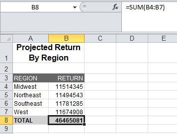
The following example illustrates how a column total in a report request is translated to an Excel formula when you use the XLSX FORMULA format. Notice that the formatting of the column total (TYPE=GRANDTOTAL) is retained in the Excel workbook. When you select the total in the report, the equation =SUM(B4:B7) displays in the formula bar, representing the column total as a sum of cell ranges.
TABLE FILE GGSALES
HEADING
"Projected Return By Region"
" "
SUM DOLLARS AS 'RETURN'
BY REGION AS 'REGION'
ON TABLE COLUMN-TOTAL
ON TABLE HOLD FORMAT XLSX FORMULA
ON TABLE SET STYLE *
TYPE=REPORT, GRID=OFF, FONT='ARIAL', SIZE=9, TITLETEXT=By Region,$
TYPE=TITLE, BACKCOLOR=RGB(102 102 102), COLOR=RGB(255 255 255),$
TYPE=HEADING, SIZE=12, STYLE=BOLD, JUSTIFY=CENTER,$
TYPE=GRANDTOTAL, BACKCOLOR=RGB(210 210 210), STYLE=BOLD,$
ENDSTYLE
END
The output is:
FOCUS can translate any total (subtotal, row total, or column total) to an Excel formula. For related information, see Translation Support for FORMAT XLSX FORMULA.
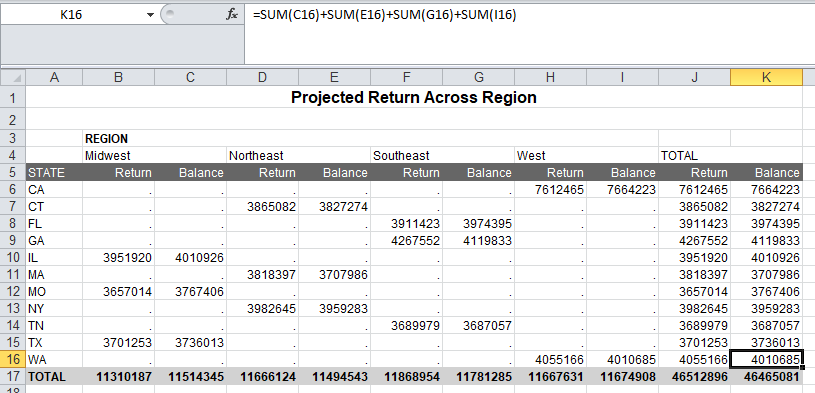
Example: Generating Native Excel Formulas for Row Totals
The following request calculates totals across regions. The row totals are represented as sums of cell ranges.
TABLE FILE GGSALES
HEADING
"Projected Return Across Region"
" "
SUM BUDDOLLARS AS 'Return' AND
DOLLARS AS 'Balance'
BY ST AS 'STATE'
ACROSS REGION AS 'REGION'
ON REGION ROW-TOTAL AS 'TOTAL'
ON TABLE COLUMN-TOTAL AS 'TOTAL'
ON TABLE HOLD FORMAT XLSX FORMULA
ON TABLE SET STYLE *
TYPE=REPORT, GRID=OFF, FONT='ARIAL',
SIZE=9, TITLETEXT=Across Region,$
TYPE=TITLE, BACKCOLOR=RGB(102 102 102),
COLOR=RGB(255 255 255),$
TYPE=HEADING, SIZE=12, STYLE=BOLD,
JUSTIFY=CENTER,$
TYPE=ACROSSTITLE, STYLE=BOLD,$
TYPE=GRANDTOTAL, BACKCOLOR=RGB(210 210 210),
STYLE=BOLD,$
ENDSTYLE
END
The following output highlights the formula that calculates the row total in cell K16=C16+E16+G16+I16.
Example: Generating Native Excel Formulas for Calculated Values
The following request totals the columns for BUDDOLLARS and DOLLARS, and calculates the value of a field called PROFIT by subtracting the DOLLARS from the BUDDOLLARS.
The formula for the calculated values is generated by translating the internal form of the FOCUS expression (PROFIT/D12.2MC = BUDDOLLARS - DOLLARS;) into an Excel formula. In this example, the formulas appear in cells B8, C8, and D8.
All fields referenced in the calculation should be displayed in the report for a valid formula to be created using cell references. Otherwise, it may be created using values not in the report. If the fields used in the calculation are not present in the report and there is a subsequent RECOMPUTE, the formula created for the RECOMPUTE will not be correct.
TABLE FILE GGSALES
ON TABLE SET PAGE-NUM OFF
SUM BUDDOLLARS/I8MC AND DOLLARS/I8MC
COMPUTE PROFIT/D12.2MC = BUDDOLLARS - DOLLARS;
BY REGION
HEADING
"Profit By Region"
" "
ON TABLE COLUMN-TOTAL
ON TABLE HOLD FORMAT XLSX FORMULA
ON TABLE SET STYLE *
TYPE=REPORT, GRID=OFF, FONT='ARIAL', SIZE=9, TITLETEXT=’By Region’,$
TYPE=TITLE, BACKCOLOR=RGB(102 102 102), COLOR=RGB(255 255 255),$
TYPE=HEADING, SIZE=12, STYLE=BOLD, JUSTIFY=CENTER,$
TYPE=GRANDTOTAL, BACKCOLOR=RGB(210 210 210), STYLE=BOLD,$
END
The following output highlights the formula that calculates for the column total of PROFIT: D8=SUM(D4:D7).
Example: Generating a Native Excel Formula for a Function
The following example illustrates how functions are translated to Excel reports. The function IMOD divides ACCTNUMBER by 1000 and returns the remainder to LAST3_ACCT. The Excel formula corresponds to =TRUNC((MOD($C3,(1000)))). TRUNC is used when the answer returned from an equation is being placed into an Integer field, to be sure there are no decimals.
TABLE FILE EMPLOYEE
PRINT ACCTNUMBER AS 'Account Number'
COMPUTE LAST3_ACCT/I3L = IMOD(ACCTNUMBER, 1000, LAST3_ACCT);
BY LAST_NAME AS 'Last Name'
BY FIRST_NAME AS 'First Name'
WHERE (ACCTNUMBER NE 000000000) AND (DEPARTMENT EQ 'MIS');
ON TABLE HOLD FORMAT XLSX FORMULA
ON TABLE SET STYLE *
TYPE=REPORT, GRID=OFF, FONT='ARIAL', SIZE=9,$
TYPE=TITLE, BACKCOLOR=RGB(102 102 102), COLOR=RGB(255 255 255), STYLE=BOLD,$
END
The output is:
Reference: Generating a Formula With Recomputed Values
Example: Generating a Formula With Recomputed Values
The following request computes the difference (DIFF) by subtracting budgeted dollars from dollar sales. The budgeted dollars field used in the expression is not included in the SUM command. The value of DIFF is recomputed on the region level.
TABLE FILE GGSALES
HEADING
"Profit By Region"
" "
SUM DOLLARS/I8CM
COMPUTE DIFF/I8CM=DOLLARS - BUDDOLLARS;
BY REGION
BY CATEGORY
ON REGION RECOMPUTE
ON TABLE HOLD FORMAT XLSX FORMULA
ON TABLE SET STYLE *
TYPE=REPORT, GRID=OFF, FONT='ARIAL', SIZE=9, TITLETEXT=’By Region’,$
TYPE=TITLE, BACKCOLOR=RGB(102 102 102), COLOR=RGB(255 255 255),$
TYPE=HEADING, SIZE=12, STYLE=BOLD, JUSTIFY=CENTER,$
TYPE=SUBTOTAL, BACKCOLOR=RGB(210 210 210),$
TYPE=GRANDTOTAL, BACKCOLOR=RGB(166 166 166), STYLE=BOLD,$
END
The output shows that the formula is subtracting a data value that is not displayed on the worksheet. It is actually the BUDDOLLARS value from the current hardcoded value, since there is no cell reference.
If you add the BUDDOLLARS column to the request, the formula can be recomputed correctly.
SUM DOLLARS/I8MC BUDDOLLARS/I8MC
The formula generated with the new SUM command contains cell references for both fields used in the calculation.
Using XLSX FORMULA With Prefix Operators
XLSX FORMULA output supports prefix operators that are used on summary lines generated by FOCUS commands, such as SUBTOTAL and RECOMPUTE. Where a corresponding formula exists in Excel, these prefix operators are translated into the equivalent Excel summarization formula. The results of prefix operators used directly against retrieved data continue to be passed to Excel as values, not formulas.
The following table identifies the prefix operators supported by XLSX FORMULA when used on summary lines, and the Excel formula equivalent placed in the generated worksheet.
|
Prefix Operator |
Excel Formula Equivalent |
|---|---|
|
SUM. |
=SUM() |
|
AVE. |
=AVERAGE() |
|
CNT. |
=COUNT() |
|
MIN. |
=MIN() |
|
MAX. |
=MAX() |
The following prefix operators are not translated to formulas when used on summary lines in XLSX FORMULA.
- ASQ.
- FST.
- LST.
Note:
- When using a prefix operator on a field
specified directly against retrieved data, there is no space between
the prefix operator and the field on which it operates.
For example, in the following aggregating display command, the AVE. prefix operator operates on the DOLLARS field.
SUM AVE.DOLLARS
- When using a prefix operator on a summary line, you must leave
a space between the prefix operator and the aggregated field on
which it operates.
In the following summary command, the MAX. prefix operator operates on the DOLLARS field at the REGION sort break. Note the required blank space between the prefix operator and the field name.
ON REGION RECOMPUTE MAX. DOLLARS
Example: Using a Summary Prefix Operator With FORMAT XLSX FORMULA
In the following request against the GGSALES data source, the RECOMPUTE command for the REGION sort field calculates the maximum of the aggregated DOLLARS field and the minimum of the aggregated BUDDOLLARS field.
TABLE FILE GGSALES
SUM UNITS DOLLARS/I8MC BUDDOLLARS/I8MC
AND COMPUTE DIFF/I8MC= DOLLARS-BUDDOLLARS;
BY REGION
BY CATEGORY
WHERE CATEGORY EQ 'Food' OR 'Coffee'
WHERE REGION EQ 'West' OR 'Midwest'
ON REGION RECOMPUTE MAX. DOLLARS MIN. BUDDOLLARS DIFF
ON TABLE HOLD FORMAT XLSX FORMULA
ON TABLE SET STYLE *
TYPE=REPORT, GRID=OFF, FONT='ARIAL', SIZE=9,$
TYPE=TITLE, BACKCOLOR=RGB(102 102 102), COLOR=RGB(255 255 255),$
TYPE=SUBTOTAL, BACKCOLOR=RGB(210 210 210),$
TYPE=GRANDTOTAL, BACKCOLOR=RGB(166 166 166), STYLE=BOLD,$
END
In the output, shown in the following image, the cell that represents the recomputed DOLLARS for the Midwest region has been generated as the following formula.
=MIN(E2:E3)
Example: Using a Prefix Operator on a Display Command With FORMAT XLSX FORMULA
In the following request against the GGSALES data source, the CNT., AVE., and PCT. Prefix operators are used in the SUM display command.
TABLE FILE GGSALES
SUM UNITS
CNT.UNITS
AVE.UNITS
PCT.UNITS
BY REGION
BY ST
ON TABLE HOLD FORMAT XLSX FORMULA
END
The output shows that the prefix operators were not passed to Excel as formulas. They were passed as data values.
NODATA With Formulas
|
Reference: |
Support for full Excel functionality requires that only valid numeric values are placed into cells that will be used for formula references.
The null value (NODATA='') is supported for calculations. When cells containing the default NODATA symbol (.) are used in a formula, they will cause a formula error.
For example:
SET NODATA=''
TABLE FILE GGSALES
SUM DOLLARS/D12CM UNITS/D12C AND ROW-TOTAL AND COLUMN-TOTAL
COMPUTE REVENUE/D12CM=DOLLARS*UNITS; AS 'Revenue'
BY LOWEST GGSALES.SALES01.CATEGORY
BY GGSALES.SALES01.PRODUCT
ACROSS REGION
ON TABLE HOLD FORMAT XLSX FORMULA
END
------------------------
SET NODATA=''
DEFINE FILE GGSALES
DOLLARMOD/D12CM MISSING ON=IF REGION GT 'V' THEN MISSING ELSE DOLLAR;
END
TABLE FILE GGSALES
SUM DOLLARMOD/D12CM UNITS/D12C AND ROW-TOTAL AND COLUMN-TOTAL
COMPUTE REVENUE/D12CM=DOLLARMOD*UNITS; AS 'Revenue'
BY REGION
BY LOWEST GGSALES.SALES01.CATEGORY
BY GGSALES.SALES01.PRODUCT
ON TABLE SET PAGE-NUM NOLEAD
ON TABLE HOLD FORMAT XLSX FORMULA
END
Reference: Usage Notes for XLSX With Formulas
- Formulas are defined within a single worksheet. They will not be assigned across worksheets.
Controlling Column Width and Wrapping in XLSX Report Output
|
How to: |
- Column width and data wrapping can be controlled in an Excel worksheet when using FORMAT XLSX.
- To size the column without wrapping and define the exact size width, use SQUEEZE=ON. If a data value is wider than the specified width of the column, a portion of the data will be hidden from view, but fully visible in the formula bar. You can adjust the column width in Excel after the worksheet has been generated.
- The default behavior is for all data to wrap within the defined column width. You can also specify the exact width of a column using WRAP=ON.
- WRAP is not supported for Date format fields.
Syntax: How to Set Column Width in XLSX Report Output
TYPE=REPORT, [COLUMN=column,] SQUEEZE=value,$
where:
- column
-
Identifies a particular column. If COLUMN is not included in the declaration, default SQUEEZE behavior is applied to the entire report.
- value
-
Is one of the following:
- ON
-
Automatically sizes the columns based on the largest data value in the column. This is the default behavior.
- OFF
-
Sizes the columns based on the maximum size defined for the field in the Master File or Define.
- n
-
Represents a specific numeric value for which the column width can be set. The value represents the measure specified with the UNITS parameter (the default is inches). This is the most commonly used SQUEEZE setting in an XLSX report. This turns off data wrapping.
Note:
- SQUEEZE can be applied to the entire report by using the ON TABLE SET SQUEEZE ON command.
- SQUEEZE is not supported for columns created with the OVER phrase or with TABLEF.
Syntax: How to Wrap Data in XLSX Report Output
TYPE=REPORT, [COLUMN=column,] WRAP=value,$
where:
- column
-
Designates a particular column to apply wrapping behavior to. If COLUMN is not included in the declaration, wrapping will be applied to the entire report.
- value
-
Is one of the following:
- ON
-
Turns on data wrapping. ON is the default value. With this setting, the column width is determined by the client (Excel). Data wraps if it exceeds the width of the column and the row height expands to meet the new height of the wrapped data.
- OFF
-
Turns off data wrapping. Data will not wrap in any cell in the column.
- n
-
Represents a specific numeric value that the column width can be set to. The value represents the measure specified with the UNITS parameter (the default is inches).
This setting implies ON. However, the column width is set to the specified width unless the data is wider than the column width, in which case, wrapping will occur as for ON.
Note: WRAP is not supported for Date format fields.
Example: Controlling Column Width and Wrapping in XLSX Report Output
The following example illustrates how to turn on and turn off data wrapping in a column and how to set the column width for a particular column. The UNITS in this example are set to inches (the default).
DEFINE FILE GGSALES
PROFIT/D14.3 = BUDDOLLARS-DOLLARS;
DESCRIPTION/A80 = 'Subtract Total Sales Quota from Reported Sales to calculate profit.';
END
TABLE FILE GGSALES
SUM
DESCRIPTION AS 'DEFAULT'
DESCRIPTION AS 'WRAP = 2'
DESCRIPTION AS 'WRAP = OFF'
DESCRIPTION AS 'SQUEEZE = 1.5'
PROFIT
BY REGION NOPRINT
ON TABLE HOLD FORMAT XLSX
ON TABLE SET STYLE *
TYPE=REPORT, COLUMN=DESCRIPTION(2), WRAP=2,$
TYPE=REPORT, COLUMN=DESCRIPTION(3), WRAP=OFF,$
TYPE=REPORT, COLUMN=DESCRIPTION(4), SQUEEZE=1.5,$
END
where:
- The column titled "DEFAULT" illustrates the default column width and wrapping behavior.
- The column titled "WRAP=2" sets the column width to 2 inches with data wrapping on.
- The column titled "WRAP=OFF" turns off data wrapping for that column.
- The column titled "SQUEEZE=1.5" sets the column width to 1.5 inches with data wrapping off.
Since the output spans two pages, the output is shown below in two separate images.
The following output displays the different behavior for the "DEFAULT" and "WRAP=2" columns.
The following output displays the output for the "WRAP=OFF" and "SQUEEZE=1.5" columns.
Preserving Leading and Internal Blanks in Report Output
|
How to: |
The SHOWBLANKS command allows you to preserve leading blanks in data cells and headings in XLSX reports. In XLSX, internal blanks will always be retained, but leading and trailing blanks in data fields are removed. You can use the SHOWBLANKS command to retain leading and trailing blanks.
Since XLSX is not HTML-based like EXL2K, setting SHOWBLANKS OFF will not affect internal blanks. By default, EXL2K reduces all embedded blanks to a single blank, while XLSX preserves all embedded blanks. This difference in spacing may cause additional differences in how fields wrap within a cell.
|
SET SHOWBLANKS |
XLSX (not HTML-based) |
EXL2K (HTML-based) |
|
SET SHOWBLANKS = ON |
Leading and embedded blanks are preserved. |
Leading and embedded blanks are preserved. |
|
SET SHOWBLANKS = OFF |
Leading blanks are removed, but embedded blanks are respected. |
Leading and embedded blanks are removed. |
Blanks are handled differently in headings:
- By default, in standard headings containing multiple items (without HEADALIGN=BODY), items are concatenated together into a single text object. All blanks are retained.
- Fields placed in headings with HEADALIGN=BODY behave the same way as data elements.
- Variables placed in headings with HEADALIGN=BODY respect all leading, embedded blanks, and trailing blanks. With SHOWBLANKS=OFF, only embedded blanks are retained. With SHOWBLANKS=ON all leading, embedded, and trailing blanks are retained.
Syntax: How to Preserve Leading and Internal Blanks in XLSX Reports
In a FOCEXEC or in a profile, use the following syntax:
SET SHOWBLANKS = {OFF|ON}
In a request, use the following syntax
ON TABLE SET SHOWBLANKS {OFF|ON}
where:
- OFF
-
Removes leading blanks and preserves internal blanks in XLSX report output. OFF is the default value.
- ON
-
Preserves leading and internal blanks in XLSX report output. Also preserves trailing blanks in heading, subheading, footing, and subfooting lines that use the default heading or footing alignment.
Example: Preserving Leading and Internal Blanks in XLSX Report Output
The following request creates a variable called SHOWVAR that contains leading, internal, and trailing blanks.
SET SHOWBLANKS = OFF

-SET &SHOWVAR= '  AB  C  ';
DEFINE FILE CAR
SHOWFIELD/A9 = '  AB  C  ';
END

TABLE FILE CAR
ON TABLE SUBHEAD
"SHOWBLANKS OFF"
"/&SHOWVAR/"
""
HEADING
"In Heading:"
"SHOWVAR<+0>&SHOWVAR"
"SHOWFIELD<+0><SHOWFIELD"
""
"In DATA":
PRINT SHOWFIELD
BY COUNTRY
WHERE RECORDLIMIT EQ 1;
ON TABLE HOLD FORMAT XLSX
ON TABLE SET STYLE *
HEADALIGN=BODY,SQUEEZE=ON,$
TYPE=TABHEADING,COLSPAN=2,$
END
The following outputs show the differences in XLSX generated using SET SHOWBLANKS = OFF and SET SHOWBLANKS = ON.
SET SHOWBLANKS = OFF with HEADALIGN=BODY (no leading blanks or trailing blanks)
SET SHOWBLANKS = OFF without HEADALIGN=BODY (preserved blanks and concatenated heading items)
SET SHOWBLANKS = ON with HEADALIGN=BODY (leading blanks and trailing blanks)
SET SHOWBLANKS = ON without HEADALIGN=BODY (preserved blanks and concatenated heading items)
Excel Page Settings
|
How to: |
Excel page settings for the XLSX workbook default to the FOCUS standards:
- Orientation: Portrait
- Page Size: Letter
- ,75 inches (Excel default)
- .75 inches (Excel default)
To customize these page settings, turn the XLSXPAGESETS attribute ON and define individual attributes.
If XLSXPAGESETS is turned on, but the page margin attributes are not defined within the procedure, the values will be set to the FOCUS default of .25 inches.
Syntax: How to Define Excel Page Settings
[TYPE=REPORT,] XLSXPAGESETS={ON|OFF} [,PAGESIZE={pagesize|LETTER}]
 [,ORIENTATION={PORTRAIT|LANDSCAPE}] [,TOPMARGIN=n] [,BOTTOMMARGIN=m],$
where:
- XLSPAGESETS={ON|OFF}
-
ON causes the page settings defined in the FOCUS request to be applied to the Excel worksheet page settings. OFF retains the default page settings defined in the standard Excel workbook. OFF is the default value.
- n
-
Defines the top margin for the worksheet in the units identified by the UNITS parameter (inches, by default). The default value is .25.
- m
-
Defines the bottom margin for the worksheet in the units identified by the UNITS parameter (inches, by default). The default value is .25.
- pagesize
-
Is one of the PAGESIZE values supported in a FOCUS StyleSheet. LETTER is the default page size.
- PORTRAIT|LANDSCAPE
-
PORTRAIT displays the report across the narrower dimension of a vertical page, producing a page that is longer than it is wide. PORTRAIT is the default value.
LANDSCAPE displays the report across the wider dimension of a horizontal page, producing a page that is wider than it is long.
Adding an Image to a Report
|
In this section: |
FOCUS supports the placement of images within each area or node of the report on the worksheet. An image, such as a logo, gives corporate identity to a report, or provides visual appeal. Data specific images can be placed in headers, footers, and data columns to provide additional clarity and style.
The image must reside in an APP or a sequential file, or be a member in a data set. If the image is not in an APP, the sequential file or member must be allocated, and you can use the DDNAME or file name as the image name.. If the file is not on the search path, supply the full path name.
Inserting Images Into Excel XLSX Reports
|
How to: |
Images can be placed in any available FOCUS reporting node or element of a worksheet. Supported image formats include .gif and .jpg.
Usage Considerations
- All images will be placed in the top-left corner of the first cell of the defined area, based on the top and left gap. Defined explicit positioning and justification have not been implemented yet.
- Standard page setting keywords can be used in conjunction with XLSXPAGESETS to control the page layout in standard reports (not compound).
- Images placed within a report cell in a row or column are anchored to the top-left corner of the cell. The cell is automatically sized to the height and width to fit the largest image (SQUEEZE=ON).
- Additional lines may need to be added within a heading, footing, subhead, or subfoot to accommodate the placement of the image.
Syntax: How to Insert Images Into FOCUS Report Elements in XLSX Reports
TYPE={REPORT|heading|data}, IMAGE={url|file|(column)} [,BY=byfield] [,SIZE=(w h)] ,$
where:
- REPORT
-
Embeds an image in the body of a report. The image appears in the background of the report. REPORT is the default value.
- heading
-
Embeds an image in a heading or footing. Valid values are TABHEADING, TABFOOTING, FOOTING, HEADING, SUBHEAD, and SUBFOOT. Provide sufficient blank space in the heading or footing so that the image does not overlap the heading or footing text. You may also want to place heading or footing text to the right of the image using spot markers.
- data
-
Defines a cell within a data column to place the image. Must be used with COLUMNS= attributes to identify the specific report column where the image should be anchored.
- url
-
Is the URL of the image file.
- file
-
Is the name of the image file. The image file or member must be allocated, and you can specify the DDNAME or, if the image is in a sequential file, the file name. If the image is in an APP, you can use the appname/filename syntax. When specifying a GIF file, you can omit the file extension.
- column
-
Is an alphanumeric field in the data source that contains the name of an image file. Enclose the column in parentheses ( ). The field containing the file name or image must be a display field or BY field referenced in the request. Note that the value of the field is interpreted exactly as if it were typed as the URL of the image in the StyleSheet. If you omit the suffix, .GIF is supplied, by default. You can use the SET BASEURL command for supplying the base URL of the images. This way, the value of the field does not have to include the complete URL. This syntax is useful, for example, if you want to embed an image in a SUBHEAD, and you want a different image for each value of the BY field on which the SUBHEAD occurs.
- byfield
-
Is the sort field that generates the subhead or subfoot.
- SIZE
-
Is the size of the image. By default, an image is added at its original size.
- w
-
Is the width of the image, expressed in the unit of measurement specified by the UNITS parameter. Enclose the w and h values in parentheses. Do not include a comma between them.
- h
-
Is the height of the image, expressed in the unit of measurement specified by the UNITS parameter.
Example: Adding a GIF Image to a Single Table Request
DYNAM ALLOC DD GIF1 DA USER1.GGLOGO.GIF SHR REU
DYNAM ALLOC DD GIF2 DA USER1.LOGO.GIF SHR REU
DEFINE FILE GGSALES
SHOWCAT/A100=CATEGORY || '.GIF';
END
TABLE FILE GGSALES
SUM DOLLARS/D12CM UNITS/D12C
BY LOWEST CATEGORY NOPRINT
BY SHOWCAT NOPRINT
BY PRODUCT
ACROSS REGION
WHERE CATEGORY NE 'Gifts'
ON CATEGORY SUBHEAD
" "
“Image in SUBHEAD for Category <CATEGORY "
" "
ON TABLE SUBHEAD
" "
" "
" Report Heading "
" "
ON CATEGORY SUBFOOT
"ON CATEGORY SUBFOOT"
ON TABLE SUBFOOT
"Report Footing"
" "
ON TABLE SET PAGE-NUM NOLEAD
ON TABLE NOTOTAL
ON TABLE SET ACROSSTITLE SIDE
ON TABLE HOLD FORMAT XLSX
ON TABLE SET STYLE *
TYPE=REPORT, GRID=OFF, FONT='ARIAL', SIZE=9, TITLETEXT='Food and Coffee',$
TYPE=REPORT, COLUMN=PRODUCT, SQUEEZE=1,$
TYPE=TITLE, BACKCOLOR=RGB(90 90 90), COLOR=RGB(255 255 255), STYLE=BOLD,$
TYPE=ACROSSTITLE, STYLE=BOLD, BACKCOLOR=RGB(90 90 90),
COLOR=RGB(255 255 255),$
TYPE=ACROSSVALUE, BACKCOLOR=RGB(218 225 232), STYLE=BOLD, JUSTIFY=CENTER,$
TYPE=HEADING, STYLE=BOLD, COLOR=RGB(0 35 95), SIZE=12, JUSTIFY=Center,$
TYPE=FOOTING, BACKCOLOR=RGB(90 90 90), SIZE=12, COLOR=RGB(255 255 255), STYLE=BOLD, JUSTIFY=CENTER,$
TYPE=SUBHEAD, SIZE=12, STYLE=BOLD, BACKCOLOR=RGB(218 225 232), JUSTIFY=CENTER,$
TYPE=SUBHEAD, IMAGE=(SHOWCAT), SIZE=(.6 .6),$
TYPE=SUBFOOT, SIZE=10, STYLE=BOLD, JUSTIFY=CENTER,$
TYPE=TABHEADING, SIZE=12, STYLE=BOLD, JUSTIFY=CENTER,$
TYPE=TABHEADING, IMAGE=gglogo.gif,$
TYPE=TABFOOTING, SIZE=12, STYLE=BOLD, JUSTIFY=RIGHT,$
TYPE=TABFOOTING, IMAGE=logo.gif, SIZE=(1.67 .6),$
END
In the following request, since the referenced images are not part of the existing GGSALES table, the image files (.gif) are being built in the DEFINE and then referenced in the TABLE request. You can NOPRINT fields if you do not want them to display as columns, but the fields must be referenced in the table to include them in the internal matrix. This will allow the images to be placed in the headings, footings, or data cells. The specific location is defined using StyleSheet definitions for attaching the image based on the field value.
Inserting Images Into XLSX Workbook Headers and Footers
|
How to: |
|
Reference: |
FOCUS supports the insertion of images into Excel headers and footers and the definition of key page settings within the Excel Worksheet Page Setup to support the placement of these images in relationship to the overall worksheet and Excel generated page breaks. This access to the Excel page functionality is designed to enhance overall usability of the worksheets for users who will be printing these reports. Page settings including orientation, page size, and page margins will directly affect the layout of each Excel page based on values defined within the FOCEXEC. Images can be included on headers and footers on every printed page, on the first page of the report only, or only on all subsequent pages. The FOCUS headings and footings continue to display within the worksheet. With this new feature, FOCUS can insert logos to be printed once at the top of a report and watermark images that need to be displayed on every printed page.
Syntax: How to Insert Images Into Excel Headers and Footers
TYPE={PAGEHEADER|PAGEFOOTER},OBJECT=IMAGE,
 IMAGE=imagename, JUSTIFY={LEFT|CENTER|RIGHT}
 [,DISPLAYON={FIRST|NOT-FIRST}]
 [,SIZE=(w h)],$
where:
- PAGEHEADER
-
Places the image in the worksheet header.
- PAGEFOOTER
-
Places the image in the worksheet footer.
- imagename
-
Is the name of a valid image file to be placed in the header or footer. The image must be available to FOCUS by being allocated to a DDNAME, and the image name in the StyleSheet must be the DDNAME. The image types supported are GIF and JPEG.
- JUSTIFY={LEFT|CENTER|RIGHT}
-
Identifies the area in the header or footer to contain the image and the justification or placement within that defined area.
- DISPLAYON
-
Defines whether the image should be placed on the first page only or on all pages except the first. Omit this attribute to place the image on all pages.
Valid values are:
FIRST places the image only on the first page.
NOT-FIRST places the image on every page except the first page.
- SIZE=(w h)
-
Is the size of the image. By default, an image is added at its original size.
w is the width of the image, expressed in the unit of measurement specified by the UNITS parameter.
h is the height of the image, expressed in the unit of measurement specified by the UNITS parameter.
Example: Inserting Images in Excel Headers and Footers and Defining Page Settings
The following request against the GGSALES data source places the image, ibi_logo.gif, on the left header area of the first page and the right header area of every other page of the resulting worksheet. It places the image webfocus1.gif in the center area of the footer on every page:
TABLE FILE GGSALES
SUM DOLLARS UNITS BUDDOLLARS BUDUNITS
BY REGION
BY ST
BY CATEGORY
BY PRODUCT
ON TABLE SET BYDISPLAY ON
ON TABLE HOLD FORMAT XLSX
ON TABLE SET STYLE *
FONT=ARIAL,SIZE=12,
XLSXPAGESETS=ON,TOPMARGIN=1,BOTTOMMARGIN=1,ORIENTATION=LANDSCAPE,
PAGESIZE=LETTER,$
TYPE=TITLE, COLOR=WHITE, BACKCOLOR=GREY,$
TYPE=PAGEHEADER, OBJECT=IMAGE, JUSTIFY=LEFT, IMAGE=IBI_LOGO.GIF, DISPLAYON=FIRST,$
TYPE=PAGEHEADER, OBJECT=IMAGE, JUSTIFY=RIGHT, IMAGE=IBI_LOGO.GIF, DISPLAYON=NOT-FIRST,$
TYPE=PAGEFOOTER, OBJECT=IMAGE, JUSTIFY=CENTER, IMAGE=webfocus1.gif, $
END
The first page of output has the image ibilogo.gif in the left area of the header and the image webfocus1.gif in the center area of the footer.
The second page of output has the image ibilogo.gif in the right area of the header and the image webfocus1.gif in the center area of the footer.
Reference: Usage Notes for Inserting Images Into XLSX Worksheet Headers and Footers
- Excel headers and footers are not automatically sized based on contents of the areas. Define page margins within the page settings to account for the space required to display the images within each page of the report.
- The image sizing based on the specified height and width is not proportional. Sizing may cause image distortion.
- BLOB image fields are not supported in this release.
Reference: Displaying Watermarks on XLSX Output
Watermark images can be placed into the Excel headers to display on every printed page of the generated worksheet.
Excel places images on the page starting in the header from left to right and then the footer from left to right. Large images placed in the header may overlap images before them in the presentation order and will overlay the previous images. For page layouts with a logo in the left area and watermark centered on the page, watermark image background should be transparent so it does not overlay the logo image.
In Excel, images are placed first on the page. All other contents of the worksheet are then placed on top of the images. Text in cells and styling such as background color and drawing objects are placed on top of the images. Excel supports transparency in drawing objects and images, but not in cell background color. BACKCOLOR will cover over images placed on the page.
Example: Placing a Watermark in an XLSX Header
The following request against the GGSALES data source uses the image internaluseonly.gif as a watermark to display in the background of every page of the worksheet. Although the image is placed in the center area of the header, it is large enough to span the entire worksheet page. It has a transparent background, so it does not cover the logo images placed at the left in the header and the center in the footer:
TABLE FILE GGSALES
SUM DOLLARS UNITS BUDDOLLARS BUDUNITS
BY REGION
BY ST
BY CATEGORY
BY PRODUCT
ON TABLE SET BYDISPLAY ON
ON TABLE HOLD FORMAT XLSX
ON TABLE SET STYLE *
XLSXPAGESETS=ON,
TOPMARGIN=1,BOTTOMMARGIN=1,LEFTMARGIN=1, RIGHTMARGIN=1, ORIENTATION=LANDSCAPE,PAGESIZE=LETTER,$
TYPE=PAGEHEADER, OBJECT=IMAGE, JUSTIFY=LEFT, IMAGE=IBI_LOGO.GIF, DISPLAYON=FIRST, $
TYPE=PAGEHEADER, OBJECT=IMAGE, JUSTIFY=CENTER, IMAGE=INTERNALUSEONLY.GIF, $
TYPE=PAGEFOOTER, OBJECT=IMAGE, JUSTIFY=RIGHT, IMAGE=WEBFOCUS1.GIF, $
END
The first page of the generated worksheet shows the watermark image beneath the data. This image is displayed on every page of the worksheet.
Creating Excel Table of Contents Reports
|
In this section: |
|
How to: |
|
Reference: |
Excel Table of Contents (BYTOC) enables you to generate a separate worksheet within an instance of the report for each value of the first BY field in the FOCUS report.
Syntax: How to Use the Excel Table of Contents Feature
ON TABLE HOLD FORMAT XLSX BYTOC
Since a BYTOC report generates separate worksheets according to the value of the first BY field in the report, the report must contain at least one BY field. The primary BY field may be a NOPRINT field.
Example: Creating a Simple BYTOC Report
The following request against the GGSALES data source creates separate tabs based on the REGION sort field.
TABLE FILE GGSALES
SUM UNITS/D12C DOLLARS/D12CM
BY REGION NOPRINT
BY CATEGORY
BY PRODUCT
HEADING
"<REGION Region Sales"
ON TABLE HOLD FORMAT XLSX BYTOC
ON TABLE SET BYDISPLAY ON
ON TABLE SET STYLE *
TYPE=REPORT, FONT=ARIAL, SIZE=9,$
TYPE=HEADING, SIZE=12,$
TYPE=TITLE, BACKCOLOR=GREY, COLOR=WHITE,$
ENDSTYLE
END
The output is:
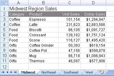
Reference: How to Name Worksheets
- The worksheet tab names are the BY field values that correspond to the data on the current worksheet. If the user specifies the TITLETEXT keyword in the StyleSheet, it will be ignored.
- Excel limits the length of worksheet titles to 31 characters. The following special characters cannot be used: ':', '?', '*', and '/'.
- If you want to use date fields as the bursting BY field, you can include the - character instead of the / character. The - character is valid in an Excel tab title. However, if you do use the / character, FOCUS will substitute it with the - character.
Naming XLSX Worksheets With Case Sensitive Data
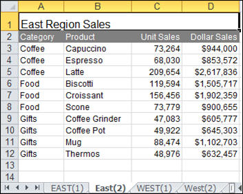
Excel requires each sheet name to be unique. Excel is case insensitive meaning it evaluates two values as being the same when the values contain the same characters but have different casing. For example, Excel evaluates the values WEST and West to be the same value. FOCUS XLSX format identifies duplicate names and adds a unique number to the name to allow Excel to maintain both sheets.
By default, FOCUS sort processing is case-sensitive, so the same field value with different casing is considered to be two different values when used as a sort (BY) field. In an Excel BYTOC report, FOCUS will generate sheets with sheet names for each value of the primary sort (BY) key based on case sensitivity. To account for this, XLSX has been enhanced to add counters where duplicate tab names are found in the data to ensure the names are unique.
For example, if the report had EAST and East as the values for the Region, each worksheet would be displayed as EAST(1) and East(2), as shown in the following image.
Overcoming the Excel 2007 and 2010 Row Limit Using Overflow Worksheets
|
How to: |
|
Reference: |
The maximum number of rows supported by Excel 2007 and 2010 on a worksheet is 1,048,576 (1MB). When you create an XLSX output file from a FOCUS report, the number of rows generated can be greater than this maximum.
To avoid creating an incomplete output file, you can have extra rows flow onto a new worksheet, called an overflow worksheet. The name of each overflow worksheet will be the name of the original worksheet appended with an increment number.
In addition, when the overflow worksheet feature is enabled, you can set a target value for the maximum number of rows to be included on a worksheet. By default, the row limit will be set to the default value for the LINES parameter (57).
Note: By default, when generating XLSX output, the FOCUS page heading and page footing commands generate only worksheet headings and worksheet footings.
Syntax: How to Enable Overflow Worksheets
Add the ROWOVERFLOW attribute to your FOCUS StyleSheet
TYPE=REPORT, ROWOVERFLOW={ON|OFF|PBON}, [ROWLIMIT={n|MAX}...
where:
- ON
-
Enables overflow worksheets.
- OFF
-
Disables overflow worksheets. OFF is the default value.
- PBON
-
Inserts FOCUS page breaks that display the page heading, footing, and column titles at the appropriate places within the worksheet rows. This option does not cause a new worksheet to start when a FOCUS page break occurs.
- ROWLIMIT=n
-
Sets a target value for the number of rows to be included on a worksheet to n rows. The default value is the LINES value (by default, 57).
- ROWLIMIT=MAX
-
Sets a target value for the number of rows to be included on a Worksheet to 1,048,000 rows for XLSX output.
This attribute works with all Excel output formats. For all other output types, the ROWOVERFLOW StyleSheet attribute is ignored, and data flow is not affected.
Reference: Usage Notes for XLSX Overflow Worksheets
- The report heading is placed once at the start of the first sheet. The report footing is placed once at the bottom of the last overflow sheet.
- Unless the PBON setting is used, worksheet headings and column titles are repeated at the top of the original sheet and each subsequent overflow sheet. Worksheet footings are placed at the bottom of the original sheet and each subsequent overflow sheet. The data values are displayed on the top data row of each overflow sheet as they would be on a standard new page.
- Report total lines are displayed at the bottom of the last overflow sheet directly above the final page and table footings.
- Subheadings, subfootings, and subtotal lines display within the data flow as normal. No special consideration is made to retain groupings within a given sheet.
- If ROWOVERFLOW=PBON, the page headings and footings and column titles display within the worksheet when a FOCUS command causes a page break.
- For XLSX output, if the ROWOVERFLOW attribute is specified in
the StyleSheet and ROWLIMIT is greater than 1MB, the following message
is presented and no output file is generated:
(FOC3338) The row limit for EXCEL XLSX worksheets is 1048576.
- Output types that contain formula references, such as XLSX FORMULA, are not supported, as formula references are not automatically updated to reflect placement on new overflow worksheets.
- The overflow worksheet feature applies to rows only, not columns. A new worksheet will not automatically be created if a report generates more than the Excel 2007/2010 limit or 16,384 columns.
- ROWOVERFLOW is supported for BYTOC reports for XLSX.
- As named ranges in Excel cannot run across multiple worksheets, the IN-RANGES phrase that defines named ranges in the resulting workbook is not supported with the ROWOVERFLOW feature. When they exist together in the same request, ROWOVERFLOW takes precedence, and the IN-RANGES phrase is ignored.
Example: Creating Overflow Worksheets
The following request creates XLSX report output with overflow worksheets. The ROWOVERFLOW=ON attribute in the StyleSheet activates the overflow feature. Without this attribute, one worksheet would have been generated instead of three.
TABLE FILE GGSALES
-* ****Report Heading****
ON TABLE SUBHEAD
"SALES BY REGION, CATEGORY, AND PRODUCT"
" "
-* ****Worksheet Heading****
HEADING
"SALES REPORT WORKSHEET <TABPAGENO"
" "
-* ****Worksheet Footing****
FOOTING
" "
"END OF WORKSHEET <TABPAGENO"
PRINT DOLLARS UNITS BUDDOLLARS BUDUNITS
BY REGION
BY CATEGORY
BY PRODUCT
BY DATE
-* ****Subfoot****
ON REGION SUBFOOT
" "
" End of Region <REGION"
" "
-* ****Subhead****
ON REGION SUBHEAD
" "
"Category <CATEGORY for Region <REGION"
" "
-* ****Report Footing****
ON TABLE SUBFOOT
" "
"END OF REPORT"
ON TABLE HOLD FORMAT XLSX
ON TABLE SET STYLE *
TYPE=REPORT, TITLETEXT=EXLOVER, ROWOVERFLOW=ON, ROWLIMIT=2000,$
ENDSTYLE
END
The report heading displays on the first worksheet only, the page heading and column titles display on each worksheet, and the subhead and subfoot display whenever the associated sort field changes value. The following image shows the top of the first worksheet, displaying the report heading, page heading, column titles, and first subhead.

Note that the TITLETEXT attribute in the StyleSheet specified the name EXLOVER, so the three worksheets were generated with the names EXLOVER1, EXLOVER2, and EXLOVER3. If there had been no TITLETEXT attribute, the sheets would have been named SHEET1, SHEET2, and SHEET3.
The worksheet footing displays at the bottom of each worksheet and the report footing displays at the bottom of the last worksheet. The following image shows the bottom of the last worksheet, displaying the last subfoot, the page footing, and the report footing.
Example: Creating Overflow Worksheets With FOCUS Page Breaks
The following request creates XLSX report output with overflow worksheets. The ROWOVERFLOW=PBON attribute in the StyleSheet activates the overflow feature, and the ROWLIMIT=250 sets the maximum number of rows in each worksheet to approximately 250. Without this attribute, one worksheet would have been generated. The PRODUCT sort phrase specifies a page break.
TABLE FILE GGSALES
-* ****Report Heading****
ON TABLE SUBHEAD
"SALES BY REGION, CATEGORY, AND PRODUCT"
" "
PRINT DOLLARS UNITS BUDDOLLARS BUDUNITS
BY REGION
BY HIGHEST CATEGORY
BY PRODUCT PAGE-BREAK
BY DATE
WHERE DATE GE '19971001'
-* ****Page Heading****
HEADING
" Product: <PRODUCT in Category: <CATEGORY for Region: <REGION"
-* ****Page Footing****
FOOTING
" "
-* ****Report Footing****
ON TABLE SUBFOOT
" "
"END OF REPORT"
ON TABLE SET BYDISPLAY ON
ON TABLE HOLD FORMAT XLSX
ON TABLE SET STYLE *
INCLUDE=endeflt,TITLETEXT=EXLOVER, ROWOVERFLOW=PBON, ROWLIMIT=250,
$
ENDSTYLE
END
The report heading displays on the first worksheet only, the page heading, footing, and column titles display on each worksheet and at each FOCUS page break (each time the product changes), and the subhead and subfoot display whenever the associated sort field changes value. The following image shows the top of the first worksheet.
Generating XLSX Compound Reports Using the OPEN, CLOSE, and NOBREAK Keywords
|
Reference: |
The keywords OPEN, CLOSE, and NOBREAK are used to control Excel compound reports. They can be specified with the HOLD command or with a separate SET COMPOUND command.
- OPEN is used on the first report of a sequence of component reports to specify that a compound report should be started.
- CLOSE is used to designate the last report in a compound report.
- NOBREAK specifies that the next report be placed on the same worksheet as the current report. If it is not present, the default behavior is to place the next report on a separate worksheet.
- When used with the HOLD syntax, the compound report
keywords OPEN, CLOSE, and NOBREAK must appear immediately after
FORMAT XLSX. For example, you can specify:
- ON TABLE PCHOLD FORMAT XLSX OPEN
- ON TABLE HOLD AS MYHOLD FORMAT XLSX OPEN NOBREAK
- As with PDF compound reports, compound report keywords can be
alternatively specified using SET COMPOUND:
- SET COMPOUND = OPEN
- SET COMPOUND = 'OPEN NOBREAK'
- SET COMPOUND = NOBREAK
- SET COMPOUND = CLOSE
Reference: Guidelines for Producing Excel Compound Reports Using XLSX
- Naming of Worksheets. The
default worksheet tab names will be Sheet1, Sheet2, and so on. You
have the option to specify a different worksheet tab name by using
the TITLETEXT keyword in the StyleSheet. For example:
TYPE=REPORT, TITLETEXT='Summary Report',$
Excel limits the length of worksheet titles to 31 characters. The following special characters cannot be used: ':', '?', '*', and '/'.
- File Names and Formats. The output
file name (AS name, or HOLD by default) is obtained from the first
report of the compound report (the report with the OPEN keyword).
Output file names on subsequent reports are ignored.
The HOLD FORMAT syntax used in the first component report in a compound report applies to all subsequent reports in the compound report, regardless of their format.
- NOBREAK Behavior. When NOBREAK is specified, the following report appears on the row immediately after the last row of the report with the NOBREAK. If additional spacing is required between the reports, a FOOTING or an ON TABLE SUBFOOT can be placed on the report with the NOBREAK, or a HEADING or an ON TABLE SUBHEAD can be placed on the following report. This allows the most flexibility, since if blank rows were added by default, there would be no way to remove them.
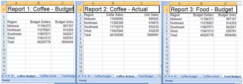
Example: Creating a Simple Compound Report Using XLSX
SET PAGE-NUM=OFF
TABLE FILE GGSALES
HEADING
"Report 1: Coffee - Budget"
" "
SUM BUDDOLLARS BUDUNITS COLUMN-TOTAL AS 'Total'
BY REGION
ON TABLE SET STYLE *
TYPE=REPORT, TITLETEXT=Coffee Budget,$
TYPE=HEADING, SIZE=14,$
ENDSTYLE
ON TABLE HOLD AS EX1 FORMAT XLSX OPEN
END
TABLE FILE GGSALES
HEADING
"Report 2: Coffee - Actual "
SUM DOLLARS UNITS COLUMN-TOTAL AS 'Total'
BY REGION
ON TABLE HOLD FORMAT XLSX
ON TABLE SET STYLE *
TYPE=REPORT, TITLETEXT=Coffee Actual,$
TYPE=HEADING, SIZE=14,$
ENDSTYLE
END
TABLE FILE GGSALES
HEADING
"Report 3: Food - Budget"
SUM BUDDOLLARS BUDUNITS COLUMN-TOTAL AS 'Total'
BY REGION
ON TABLE SET STYLE *
TYPE=REPORT, TITLETEXT=Food Budget,$
TYPE=HEADING, SIZE=14,$
ENDSTYLE
ON TABLE HOLD FORMAT XLSX CLOSE
END
The output is:
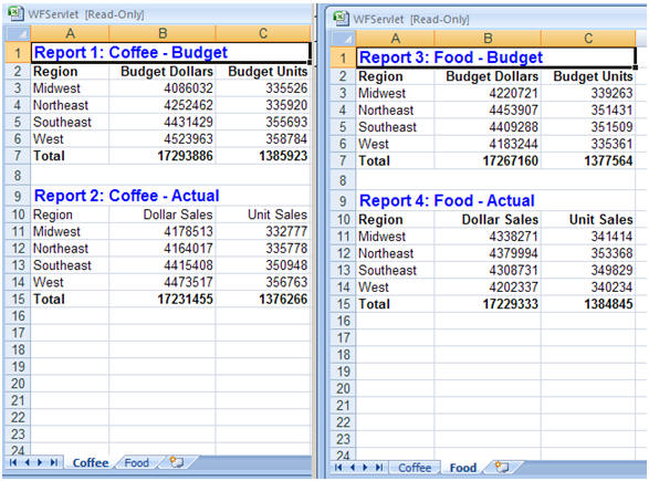
Example: Creating a Compound Report Using NOBREAK
In this example, the first two reports are on the first worksheet, and the last two reports are on the second worksheet, since NOBREAK appears on both the first and third reports.
TABLE FILE GGSALES
HEADING
"Report 1: Coffee - Budget"
SUM BUDDOLLARS BUDUNITS COLUMN-TOTAL AS 'Total'
BY REGION
IF CATEGORY EQ Coffee
ON TABLE HOLD FORMAT XLSX OPEN NOBREAK
ON TABLE SET STYLE *
TYPE=REPORT, TITLETEXT=Coffee, FONT=ARIAL, SIZE=10, STYLE=NORMAL,$
TYPE=TITLE, STYLE=BOLD,$
TYPE=HEADING, SIZE=12, STYLE=BOLD, COLOR=BLUE,$
TYPE=GRANDTOTAL, STYLE=BOLD,$
END
TABLE FILE GGSALES
HEADING
" "
"Report 2: Coffee - Actual "
SUM DOLLARS UNITS COLUMN-TOTAL AS 'Total'
BY REGION
IF CATEGORY EQ Coffee
ON TABLE HOLD FORMAT XLSX
ON TABLE SET STYLE *
TYPE=REPORT, FONT=ARIAL, SIZE=10, STYLE=NORMAL,$
TYPE=GRANDTOTAL, STYLE=BOLD,$
TYPE=HEADING, SIZE=12, STYLE=BOLD, COLOR=BLUE,$
END
TABLE FILE GGSALES
HEADING
"Report 3: Food - Budget"
SUM BUDDOLLARS BUDUNITS COLUMN-TOTAL AS 'Total'
BY REGION
IF CATEGORY EQ Food
ON TABLE HOLD FORMAT XLSX NOBREAK
ON TABLE SET STYLE *
TYPE=REPORT, TITLETEXT=Food, FONT=ARIAL, SIZE=10, STYLE=NORMAL,$
TYPE=HEADING, STYLE=BOLD, SIZE=12, COLOR=BLUE,$
TYPE=TITLE, STYLE=BOLD,$
TYPE=GRANDTOTAL, STYLE=BOLD,$
END
TABLE FILE GGSALES
HEADING
" "
"Report 4: Food - Actual"
SUM DOLLARS UNITS COLUMN-TOTAL AS 'Total'
BY REGION
IF CATEGORY EQ Food
ON TABLE HOLD FORMAT XLSX CLOSE
ON TABLE SET STYLE *
TYPE=REPORT, FONT=ARIAL, SIZE=10,  $
TYPE=TITLE, STYLE=BOLD,$
TYPE=HEADING, SIZE=12, STYLE=BOLD, COLOR=BLUE,$
TYPE=GRANDTOTAL, STYLE=BOLD,$
END
Report output is displayed in two separate tabs.
Format XLSX Limitations
Format XLSX does not support the following features currently supported for EXL2K:
- Cell Locking.
- Pivot Tables.
- Templates.