A database in a data warehouse is often organized into a "star schema," consisting of a central "fact table" with the data to be analyzed and multiple "dimension tables" that describes the data.

Each dimension table has a single surrogate key, an arbitrary unique identifier for the row. The fact table has multiple keys, each joining to a different dimension table.

Before you create and run the data flows discussed in this section, in addition to creating the source tables, you must also create the target tables. See How to Create Sample Procedures and Data for Star Schema.

This example has detailed instructions for loading one of the four dimension tables. Refer to the sample flows, DLOADCUST, DSLOADPROD, DSLOADSALE, and DSLOADTIME, for other examples of loading a dimension table. Refer to DSLOADFACT for an example of loading a fact table and DSFLOWP for the complete example of loading a star schema.

This example has instructions for loading the customer dimension table.

1. In the DMC, right-click an application directory in the navigation pane and select New, then Flow. The data flow opens in the right hand pane, with the SQL object displayed.
2. Drag the data source object DMCOMP from the ibisamp application directory in the navigation pane into the workspace, located to the left of the SQL object.
3. Right-click the SQL object and select Column Selection.

   The Column Selection window opens.

4. Right-click any column name and Select All. Then click the > arrow to add them to the selected columns and click OK.
5. Drag the target object DSDIMCUST from the ibisamp application directory into the workspace to the right of the SQL object.
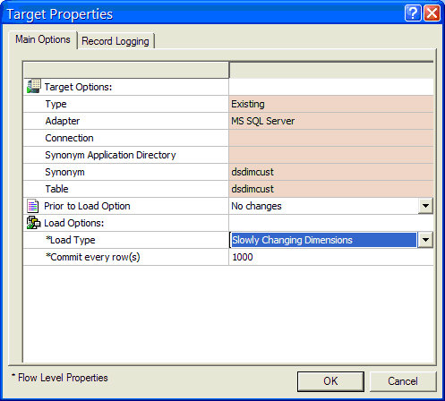
6. Right-click the target object DSDIMCUST and select Properties.

   The erties window opens.

   From the Load Type drop-down menu, select Slowly Changing Dimensions, as shown in the following image. Click OK.

   

7. Right-click the target object DSDIMCUST and select Target Transformations

   The Target Transformation window opens.

8. Click the Automap button.

   The identically named source and target column names are added to the Expressions window. The Target Transformations window should now look like the following image.

   

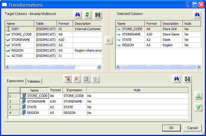
   Note: The columns CKEY and ACTIVE are not mapped because these columns are handled automatically by the DataMigrator Slowly Changing Dimension processing. CKEY is the surrogate key, which automatically starts with a value of 1 and increases by one, for each row added. The Active flag is set to 1 for currently active rows.

   Click OK to close the Transformations window.

9. From the main menu, click File, then Save. Enter dsxloadvust as the file name.

A fact table load requires looking up the keys for each row in the corresponding dimension tables, and obtaining a surrogate key so that the fact table can be joined to each of the dimensions for subsequent reporting.

To create the fact table follow these steps.

1. In the DMC, right-click an application directory in the navigation pane and choose New, then Flow. The data flow opens in the right hand pane, with the SQL object displayed.
2. Drag the data source object DMORD from the ibisamp application directory in the navigation pane into the workspace, to the left of the SQL object.
3. Drag the data source object DMSALE from the ibisamp application directory in the navigation pane into the workspace, to the left of the SQL object.

   A JOIN object is automatically added connected to DMORD[MS] and DMSALE.

4. Drag the data source object DMINV from the ibisamp application directory in the navigation pane into the workspace, to the left of the SQL object.

   A second JOIN object is automatically added connected to the first JOIN object and DMINV.

5. Right-click the SQL object and select Column Selection.

   The Column Selection window opens.

6. Select the following columns and click the > arrow to add them to the Selected Columns list:

   ORDER_DATE from DMORD(T1)

   PROD_NUM from DMINV(T3)

   STORE_CODE from DMORD(T1)

   EMPID from DMSALE(T2)

   LINEPRICE from DMORD(T1)

   QUANTITY from DMORD(T1)

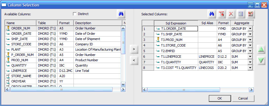
7. Click the Insert Columns button.

   The SQL Calculator opens.

8. For Alias, type LINCOGS and for calculation, expand DMPROD. Double-click QUANTITY, type*, then expand DMINV and INVINFO. Select COST so that the Expression window shows T1.QUANTITY * T3.COST.
9. Click OK to close the SQL calculator.

   The Column Selection window should appear as in the following image.

   

10. Click OK to close the Column Selection window.
11. Drag the target object DSFACT from the ibisamp application directory to the workspace to the right of the SQL object.
12. Right-click DSFACT and select Target Transformations.

    The Transformations window opens.

13. Double-click ODKEY, adding it to the Expressions window. With the line selected, click the Calculator button.

    The Transformation Calculator window opens.

14. Click the Functions tab, expand Data Source and Decoding, and double-click DB_LOOKUP.

    The Lookup function assist opens.

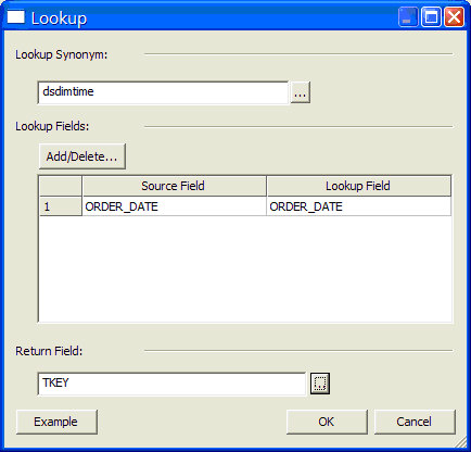
15. Click the ellipsis button after Lookup Synonym. Select the synonym DSDIMTIME from the ibisamp directory and press Enter.
16. Under Lookup fields, click the Add/Delete button. Select ORDER_DATE from the left hand side and TDATE on the right hand side. Click OK to close the dialog box.
17. Click the ellipsis button after Return Field.

    The Lookup Field dialog box opens.

18. Double-click TKEY to select it. Click OK to close the dialog box.

    The Lookup window should appear as shown in the following image.

    

19. Repeat steps 12-17 above for SHIP_DATE.
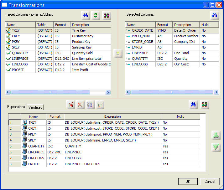
20. Similar transformations are required for each of the key columns.

    For the rest of the key columns, the Source Field and Lookup Field are pre-selected since the names are the same in the Fact and Dimension tables. In addition, transformations are required for the remaining columns.

    When you have created the remaining transformations, the Transformations window should appear as shown in the following image.

    

21. Click OK to close the window.
22. From the main menu, click File, then Save as. Enter dsloadfact as the file name.

In order to load the fact table in this example, all the dimension tables have to be loaded first so that the surrogate keys are available.

1. In the DMC, right-click an application directory in the navigation pane, select New and then Flow. The data flow opens in the right pane.
2. Click the Process Flow tab. The view switches to the process flow with a Start icon.
3. On the toolbar, click the Parallel Group button and drag it into the work area to the right of the Start icon.

   A box appears on the screen. This is an empty parallel group.

4. Right-click the Start icon and drag a line towards the parallel group box.

   Release the line when the arrow is touching the box.

5. From the Applications tab, drag the DSXLOADCUST flow inside the parallel group box. If you did not create this data flow, drag the DSLOADCUST flow from the ibisamp directory.
6. From the ibisamp directory, drag the DSLOADPROD, DSLOADSALE, and DSLOADTIME flows into the parallel group.
7. The DSLOADTIME flow requires a parameter of the first date to load. Double-click the flow to open the properties for the flow. For Parameters, enter STARTDATE=20040101.
8. On the toolbar, click the Wait button and drag it into the work area to the right of the parallel group.
9. Right-click the parallel group, drag a line to the Wait icon, and release.
10. Drag the DSXLOADFACT flow to the right of the Wait icon. If you did not create this data flow, drag the DSLOADCUST flow from the ibisamp directory.
11. Right-click the Wait icon, drag the line to the DSLOADFACT flow, and release.

    When you have finished, your process flow should appear as shown in the following image.

    

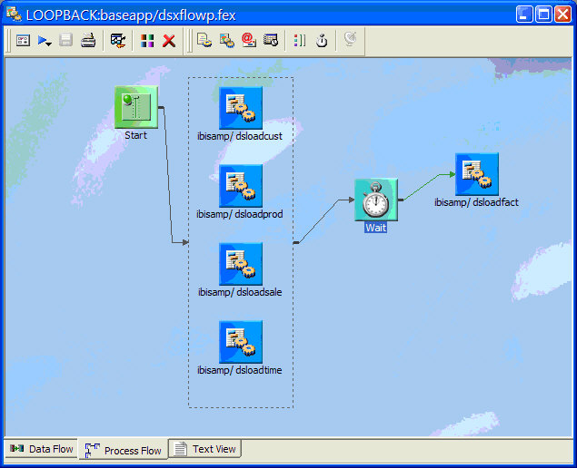
12. From the main menu, click File, then Save as. Enter dsxflowp as the file name.
13. On the toolbar, click the Run button and select Submit to run the flow.
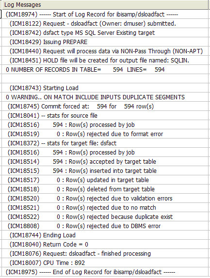
14. When the flow completes, click the View Last Log button icon.

    The process flow log opens.

    

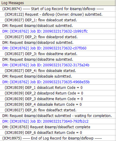
    The log shows the four dimension data flows run and the fact table load, which runs when the data flow runs are complete. The lines in blue indicate links to the detail logs for the individual flows.

15. Click the fact table log, which is the last blue line shown. The detail log opens.